27 Importance Sampling Techniques for the Analysis of Genetic Circuits

Faculty Mentor: Chris Myers (Electrical & Computer Engineering, University of Utah)

Abstract

Genetic circuits have been identified as a promising technology that could revolutionize several areas, including biofuels, biomanufacturing, and medicine. Despite the tremendous potential of this technology, there are significant challenges associated with its development and implementation. One of the major challenges with genetic circuits is the stochastic nature of their behavior. Unlike traditional engineering systems, genetic circuits are inherently probabilistic, which makes it more challenging to design and verify their performance. In particular, genetic circuits can exhibit rare failure states known as glitches, which are difficult to predict and prevent. To address this challenge, multiple stochastic simulation algorithms have been developed that use importance sampling as a variance reduction technique to estimate the probability of glitching behavior. However, these methods are often unreliable and impractical for use in design workflows. As a result, a mathematical analysis of these methods is necessary to identify the reasons why they fail to rapidly estimate low probabilities. To meet this need, we performed a comprehensive mathematical analysis of these methods to determine why they are ineffective in estimating low probabilities and to showcase their strengths and shortcomings. To achieve this end, we developed several case studies highlighting the challenges associated with these methods and their potential applications in genetic circuit design. This analysis provides crucial insights into the development of more effective algorithms for estimating the probability of rare glitching behaviors in genetic circuits. The results of this work will guide the future development of more applicable algorithms that can be used in design workflows to improve the reliability and predictability of genetic circuits. By overcoming the challenges associated with the stochastic nature of genetic circuits, these algorithms will enable the widespread adoption of genetic circuit technology in various fields, including biofuels, biomanufacturing, and medicine.

Introduction

Genetic circuits are synthetic DNA constructs which implement engineered computational or logical functions in living cells. Genetic circuits promise to revolutionize biofuels, biomanufacturing, and medicine by improving biochemical production [1]. Inspired by traditional engineering disciplines, synthetic biologists utilize designbuild- test-learn (DBTL) cycles to yield useful genetic circuits [2]. The design phase of the DBTL cycle may include modeling. Modeling steps are beneficial to the design process because they allow for design verification before any circuit is actually built, reducing the necessary number of orbits around the DBTL cycle. To be useful, models of genetic circuits must be able to accurately predict whether or not a given design will fail. Predicting genetic circuit failures can be difficult, however, because chemical reaction networks, including genetic circuits, are inherently stochastic due to the random movements of molecules [3]. This stochasticity is responsible for rare failure states in genetic circuits known as glitches, which occur with some probability and may be devastating to a biological system [4, 5].

The probability of a glitch may be estimated by simulating many system trajectories with the stochastic simulation algorithm (SSA) [6, 7]. For rare events the number of trajectories necessary to precisely estimate the probability of failure may be computationally prohibitive. The problem of estimating the probability of rare events has prompted the creation of several algorithms which utilize the statistical technique of importance sampling (IS) [8] to more rapidly estimate low probabilities. These techniques include theWeighted SSA (wSSA) [9], State-dependent Weighted SSA (swSSA) [10], and Guided wSSA [11, 12].

These algorithms have been applied applied to a few toy models [9–12], but none have been shown to be suitable for use in genetic circuit design verification. To be used in genetic design verification, an IS-based stochastic simulation algorithm must be able to accurately and precisely estimate the probability of rare failure states in genetic circuits, must be straightforward to apply, and must be sufficiently stable and robust. The existing IS-based algorithms must therefore be tested for these qualities.

To this end, we implemented each algorithm and benchmarked its performance on a number of case studies varying from toy models to genetic circuits. This revealed fundamental mathematical challenges which the algorithms fail to overcome. Equipped with these results, we formed recommendations for more robust IS schemes. Ultimately, this work may lead to effectual simulation methods which may be used in conjunction with stochastic model checking to accelerate the design of genetic circuits. Accelerated design protocols will prove crucial as genetic circuits are applied to diverse biochemical production tasks.

Background

Genetic Circuits Genetic circuits are synthetic collections of biological components, inspired by natural gene regulatory networks, which implement computational functions in living cells. Early examples of genetic circuits include the genetic toggle switch [13] and repressilator [14]. Over the past two decades, genetic circuits have evolved beyond simple operations to solve problems in diverse fields [1].

Digital logic circuits are often used as models of genetic circuits. The simplicity of this abstraction is appealing, but it neglects temporal dynamics and stochasticity. Nevertheless, digital logic models have proven useful in the design of genetic circuits. Working within the abstraction of digital logic circuits, Nielsen et al. developed Cello, a genetic design automation tool which produces circuit designs from a user-specified logic table. To validate Cello’s performance, Nielsen et al. produced 60 genetic circuits using the tool [15]. One of these circuits, 0x8E, has been shown to exhibit glitching behaviors [4, 5] and is analyzed here.

2.1 Importance Sampling

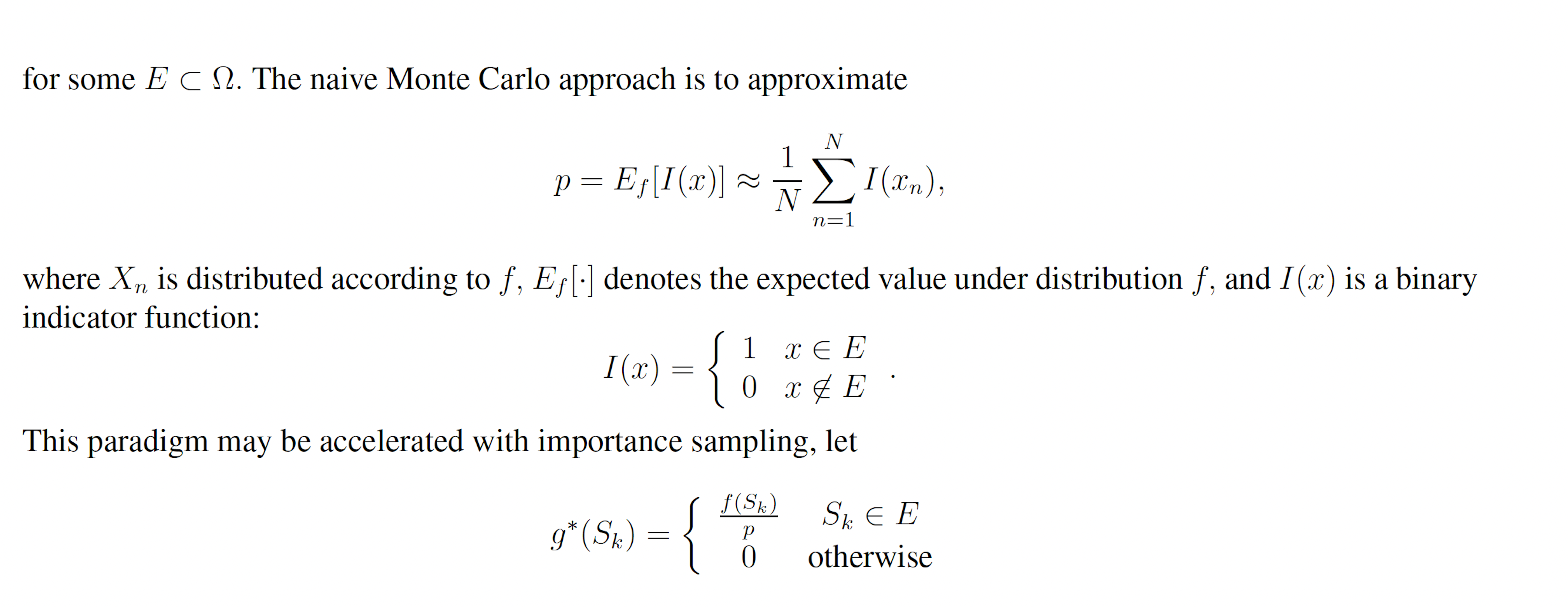
Importance sampling is a Monte Carlo technique for rapidly estimating the properties of some distribution using samples from another distribution [8]. Importance sampling, in general, operates as follows. Suppose X is a random variable with sample space Ω which is distributed according to probability density function f(x). Further suppose that we want P{X ∈ E} where P{·} denotes the probability and E ⊂ Ω. We may write

P{X ∈ E} = Ef [I(x)],

where Ef [°] denotes the expected value under distribution f and I(x) is the indicator function

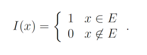
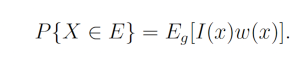
Let g(x) be a probability density function over the sample space Ω which is almost-everywhere nonzero. g is referred to as the importance density. Observe that

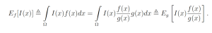Let w(x) = f(x) /  g(x) be the weight function, so we may write

By the law of large numbers,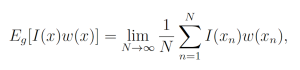

where each xn is a sample from g. This yields the unbiased estimator

which, given a good choice in g, may have lower variance than the naive sample estimator.

2.2 The SSA The SSA [6, 7] is an algorithm that produces exact trajectories of chemical reaction networks. The SSA is developed as follows. Suppose we have a chemical reaction network with n chemical species {S1, . . . , Sn} and m reactions {R1, . . . ,Rm} with corresponding reaction rate constants {a1, . . . , am} (referred to as propensity functions within the context of stochastic chemical kinetics). Let Xi(t) be a random variable representing the number of molecules of Si at time t. We write X(t) = (X1(t), . . . ,Xn(t)). Additionally, each reaction channel Rμ has an associated state-change vector vμ = (v1μ, . . . , vnμ) where viμ is the change in Xi following a turn of reaction Rμ. The state-change vectors are arranged to form the stoichiometric matrix

Let p(τ, μ|x, t)dτ denote the probability the the next reaction which occurs in a network is Rμ and that it will occur on the interval [t + τ, t + τ + dτ], given that X(t) = x. We may write

where P0(τ |x, t) denotes the probability that no reaction occurs on the interval [t, t + τ ). Observe that P0 must satisfy

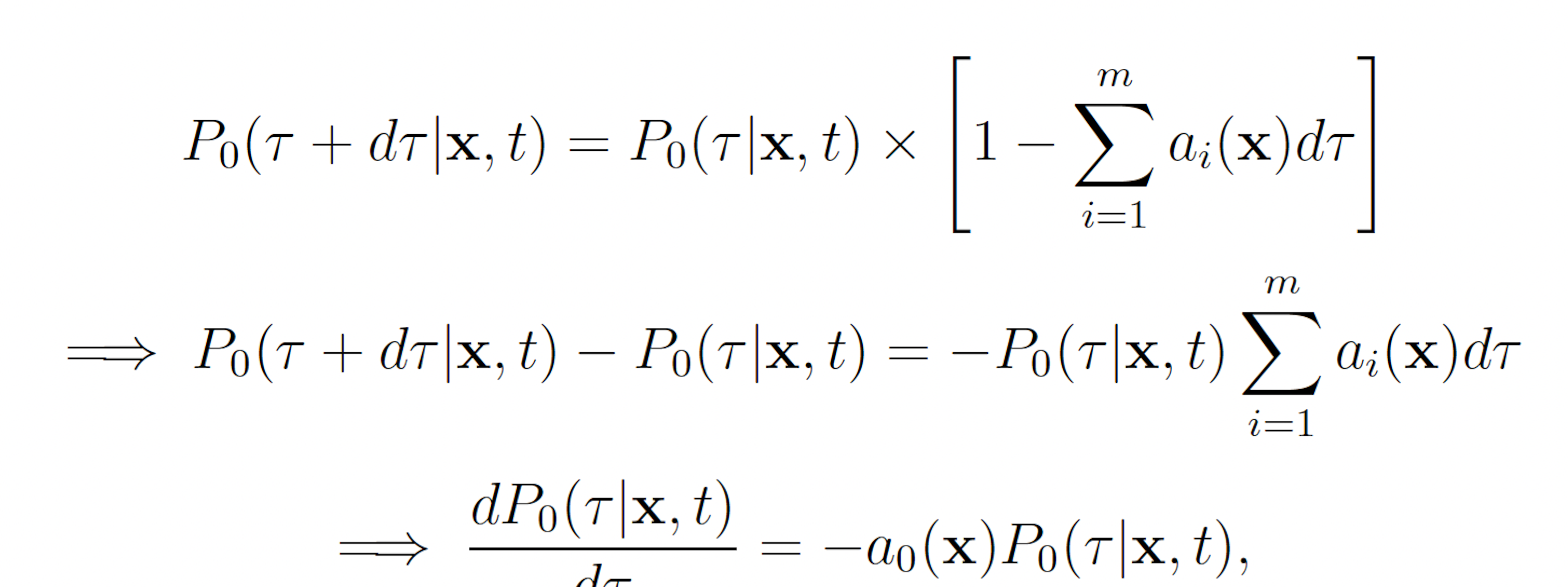
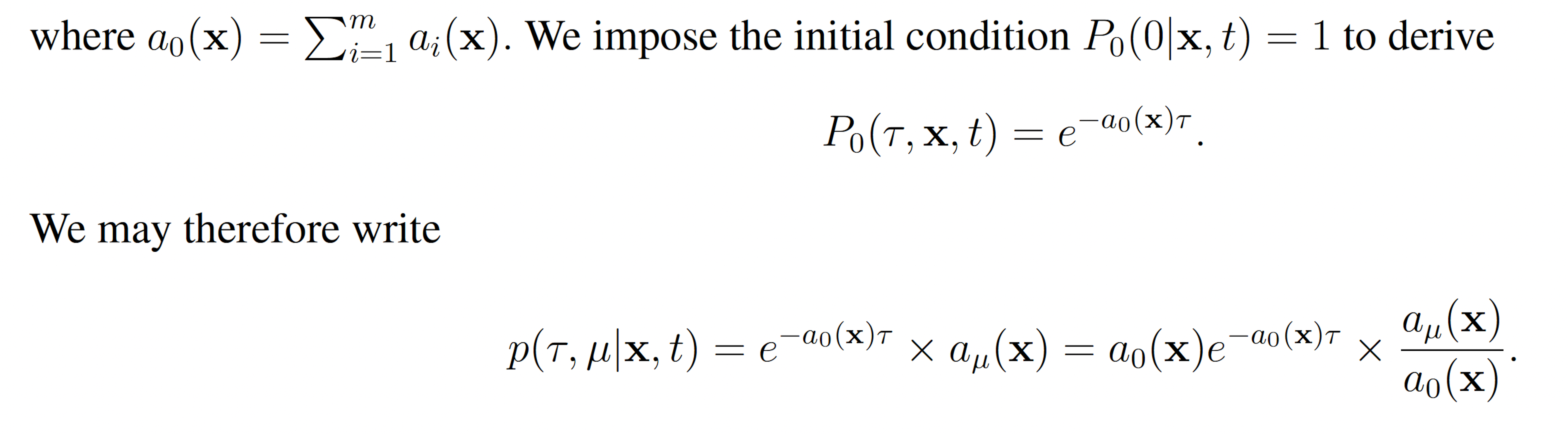
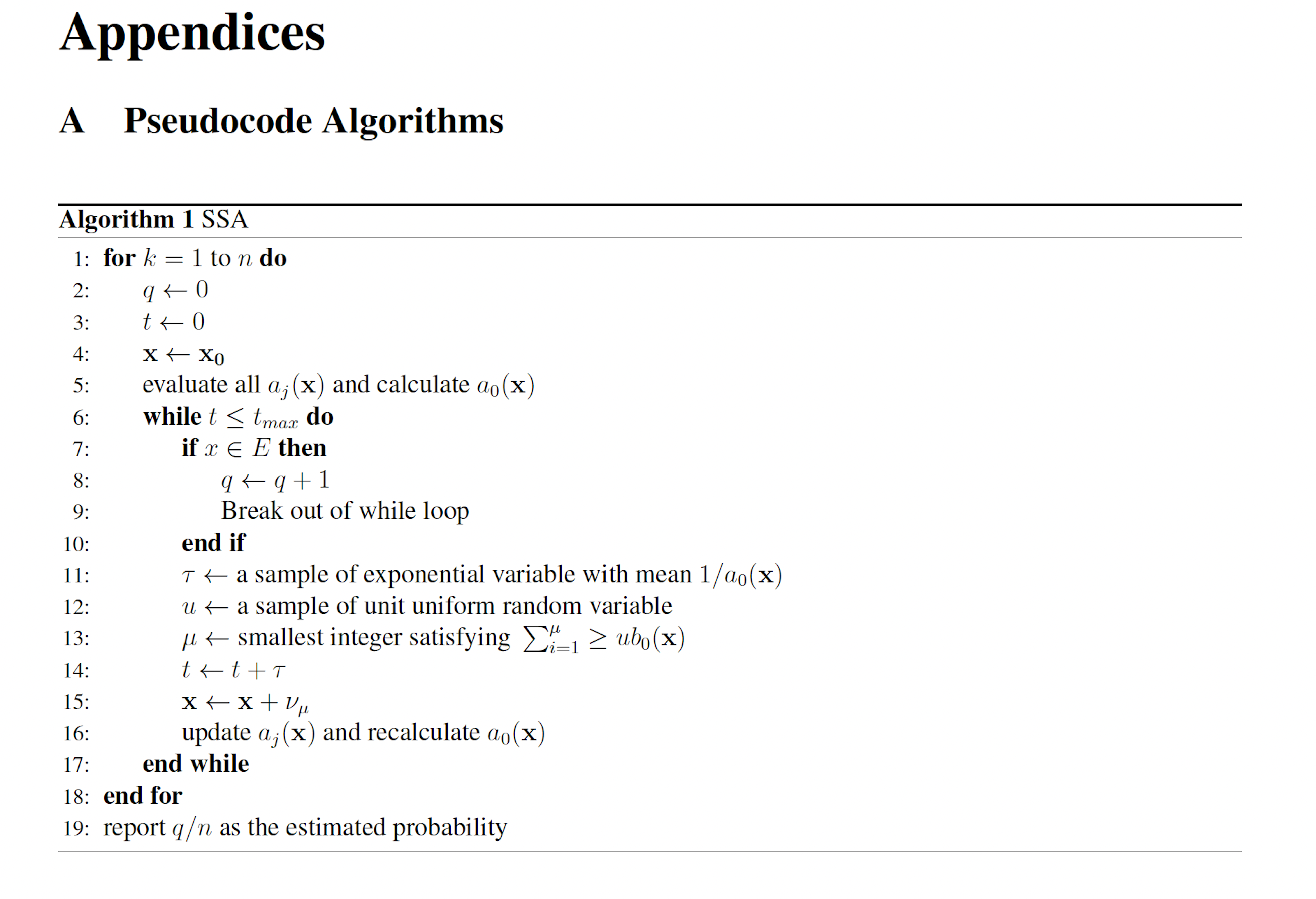
This reveals that τ and μ are independently and randomly distributed, and that τ is exponentially distributed with mean 1 a0(x) and μ is distributed such that each reaction Rμ has probability mass aμ(x)/a0(x). These observations, yield the SSA (Algorithm 1).

2.3 Weighted SSA Variants

2.3.1 The wSSA The wSSA

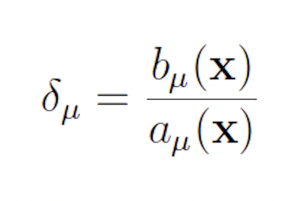
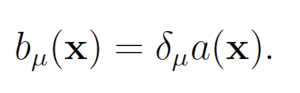
The wSSA [9] first applied IS to chemical reaction networks. The wSSA achieves this by assigning a biasing factor δμ to each reaction Rμ. These biasing factors are applied multiplicatively to the propensity functions aμ to form predilection functions

bμ(x) = δμaμ(x).

Reactions are then selected according to these predilection functions, rather than the true propensities. In the wSSA, predilection functions are not used to determine interevent time τ. Each reaction Rμ therefore has weight function

where b0(x) = Pm i=1 bi(x) If a given system trajectory has reaction sequence (Rμ(1) , . . . ,Rμ(k)), then the total weight function corresponding to the trajectory is

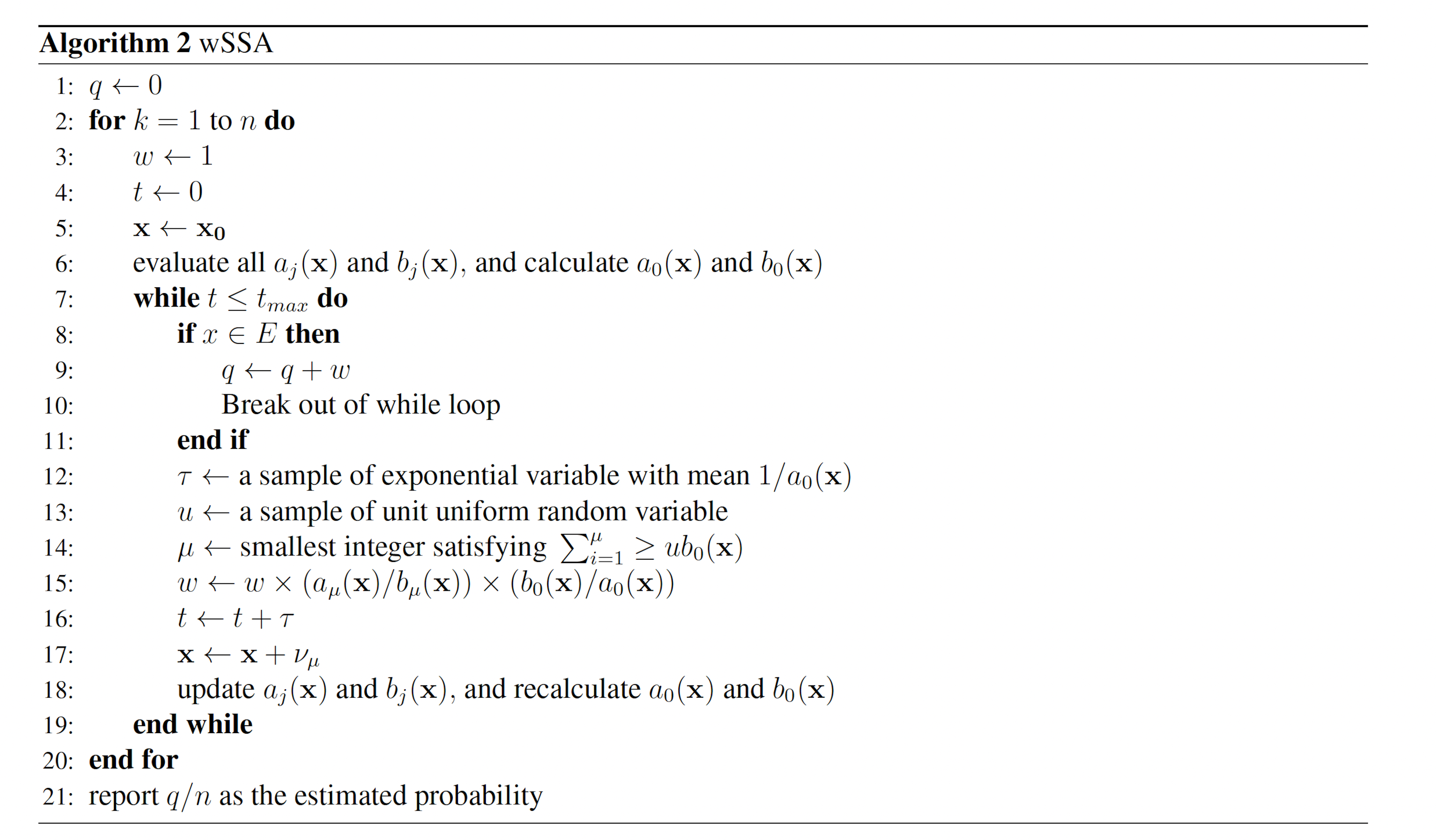
These modifications to the SSA yield the wSSA (Algorithm 2).

2.3.2 The swSSA

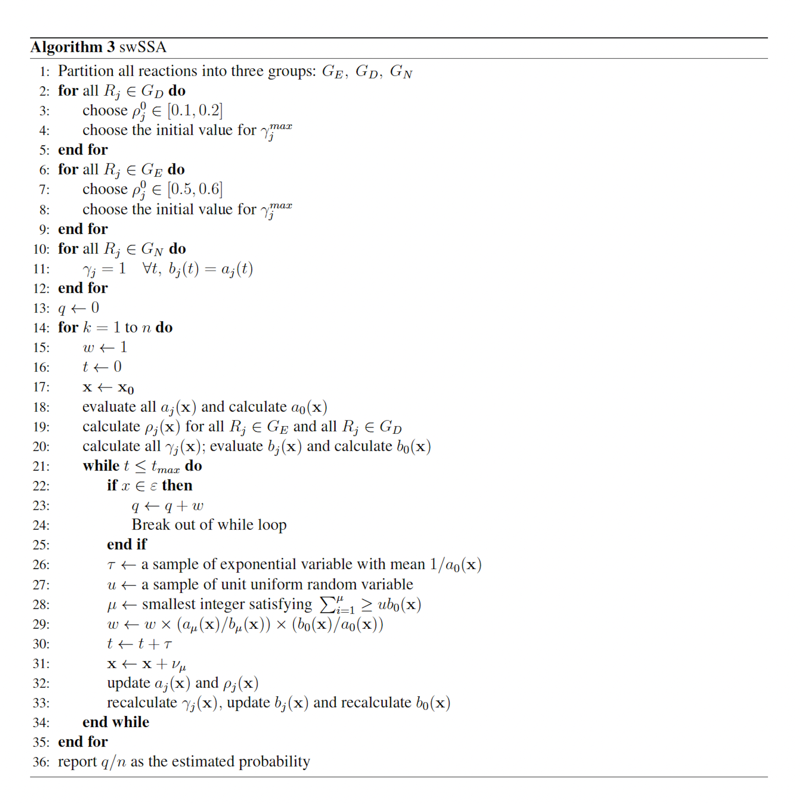
The wSSA applies constant multiplicative biasing to each propensity function to yield predilection functions [10]. This is limited because it does not account for whether the current state x causes a given propensity function aμ(x) be large or small prior to any biasing. To improve the robustness of the wSSA, the swSSA utilizes a statedependent biasing factor as follows. Let ρμ(x) = aμ(x)/a0(x) be the relative propensity. Prior to simulation, reactions to be biased upward,downward, and not at all are sorted into sets GE, GD and GN, respectively. For each reaction Rμ ∈ GE ∪ GD, a threshold ρ0 μ and maximal biasing γmax μ are selected. For Rμ ∈ GE, the dynamic multiplicative biasing factor

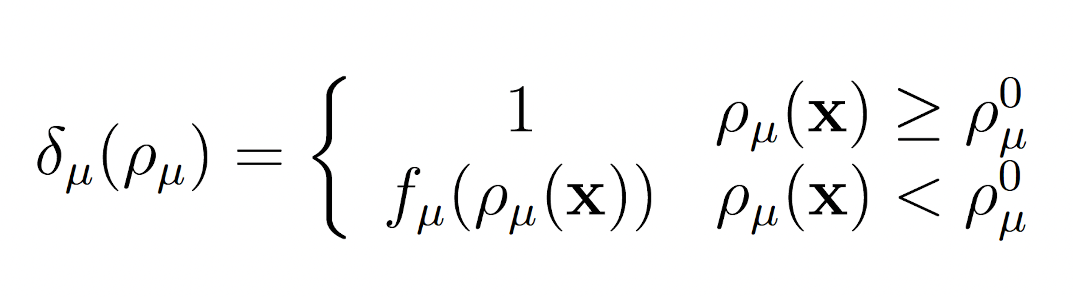
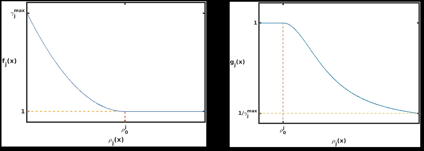
where fμ(ρμ(x)) is parabolic function with

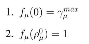
For Rμ ∈ GD, the dynamic multiplicative biasing factor

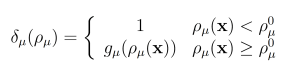
where gμ(ρμ(x)) is a parabolic function with

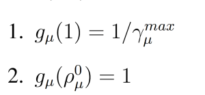
(Figure 1). These modifications to the wSSA yield the swSSA (Algorithm 3).

2.3.3 The Guided wSSA

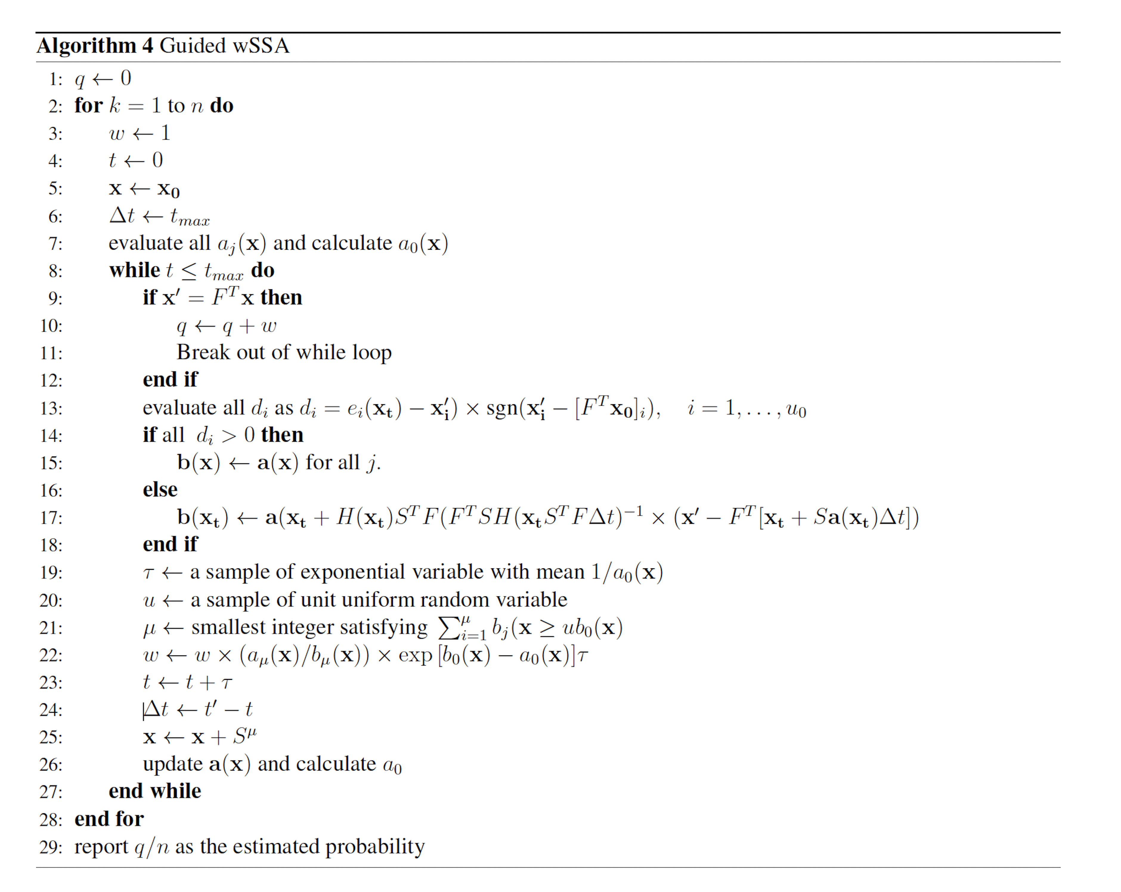
Both the wSSA and swSSA rely on the user to select biasing parameters based on some a priori knowledge of the network being simulated. The Guided wSSA [11,12] automatically biases reactions at each point in simulation to circumvent this reliance. This biasing is designed to, on average, bring the chemical reaction network to the state of interest immediately before the maximum simulation time. This is achieved by assuming that the number of times each reaction will occur before the maximum simulation time is Poisson distributed. A multivariate normal approximation to the Poisson distribution is used to calculate the expected number of times each reaction will occur before maximum simulation time given that the state of interest is reached at maximum simulation time. The details of this formulation require that the state of interest be a condition on a linear combination of chemical species, that is, there exists an F such that the state of interest is achieved when FT x reaches some value. These modifications to the wSSA yield the Guided wSSA (Algorithm 4). H denotes diag(b(x)).

Figure 1: Parabolic f and g function utilized by the swSSA.

The published version of the Guided wSSA is unstable, however, because it routinely selects negative biasing parameters, which cannot be used to select a reaction. Inspection of the original Guided wSSA implemented, provided by the authors of the Guided wSSA paper [11], reveals that three unmotivated methods were used to remove negative predilections. In all three methods, the effective biasing factors

were calculated. In one case, the 0.01 plus absolute value of the most negative biasing factor was added to all biasing factors so that all biasing factors became positive. In another case, all biasing factors were divided by the most negative biasing factor, which only eliminates negatives if all biasing factors share the same sign. In yet another case, all negative biasing factors were replaced with one. After the biasing factors were modified, the predilections were recalculated as usual:

The final method is used in analyses included in this paper.

3 Methods

3.1 Model Biochemical Systems

3.1.1 Enzymatic Futile Cycle

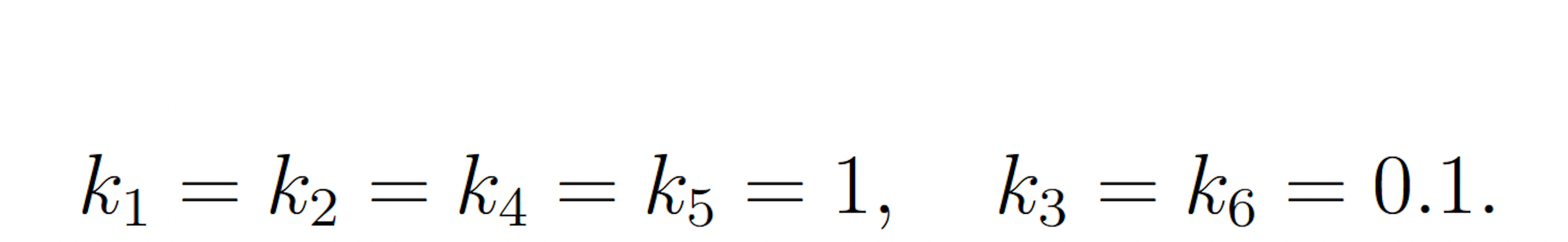
The enzymatic futile cycle is a simple biochemical motif present in a variety of biology pathways, including GTPase cycles, MAP Kinase cascades, and glucose mobilization [16]. The enzymatic futile cycle is therefore an archetypal naturally occurring biochemical system with few reactions, and is given as follows:

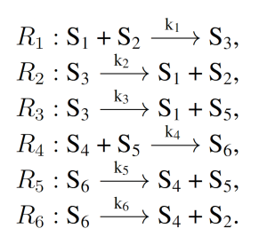
where

The rare event of interest is S5 falling to 25 molecules or fewer before 100 time units have passed, subject to the following initial conditions:

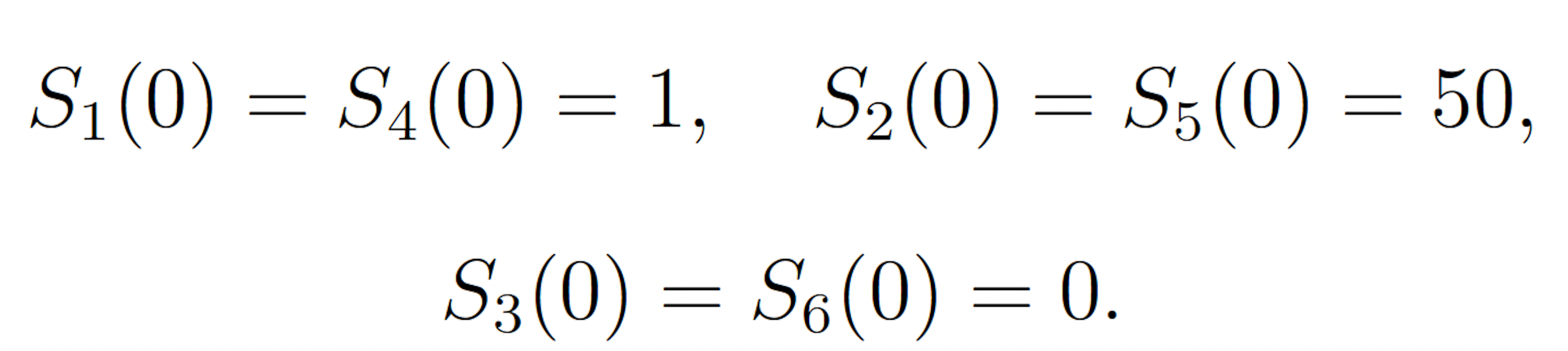
This event is rare because the symmetry of the initial molecule counts and reaction rate constants keeps the system near its initial condition with high probability. The probability of this event has been previously calculated to be 1.71 × 10−7 [9]. We consider this value to be exact.

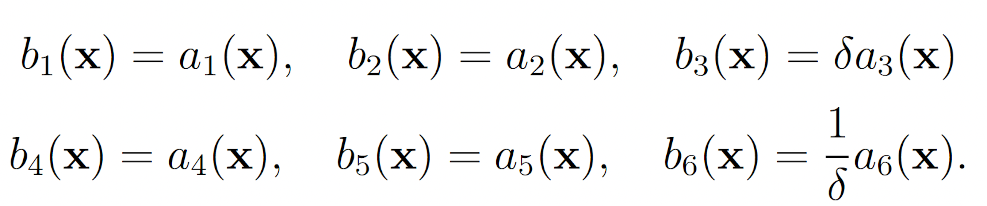
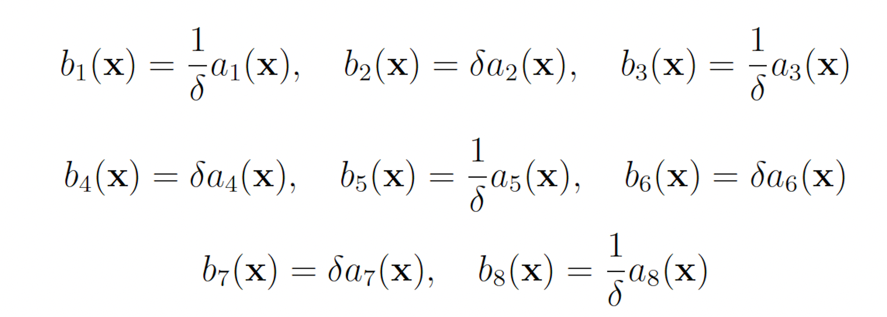
To apply the wSSA to this model, each reaction must be assigned a multiplicative biasing parameter. We used use a single biasing parameter δ ∈ (0, 1) to simplify parameter optimization to one dimension. δ was be applied to reactions to be biased downward and δ−1 was applied to reactions to be biased upward. This simplification was made for all models. In the enzymatic futile cycle, S2 production may be biased upward and S5 production may be biased downward to increase the probability of S5 falling to 25. This gives the following wSSA weighting scheme:

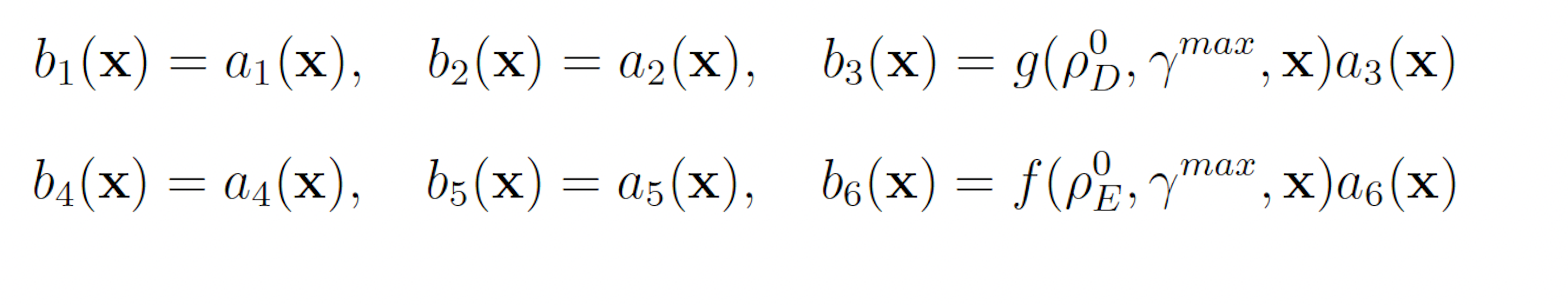
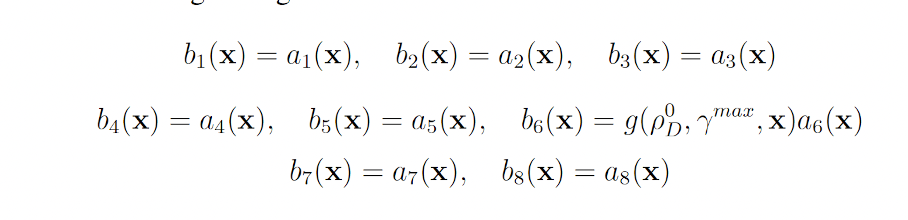
The swSSA also requires biasing parameters to be specified. Unlike the wSSA, the swSSA biases reaction in a state-dependent manner, so the user must specify a relative propensity threshold beyond which biasing is applied and a maximal biasing value. For all models, we will use a fixed threshold of ρ0 D = 0.15 for reactions that are being biased downward and ρ0 E = 0.5 for reactions that are being biased upward. The maximal biasing value γmax can then be varied to again simplify parameter optimization to one dimension. This gives the following biasing scheme for the futile cycle:

3.1.2 Modified Yeast Polarization

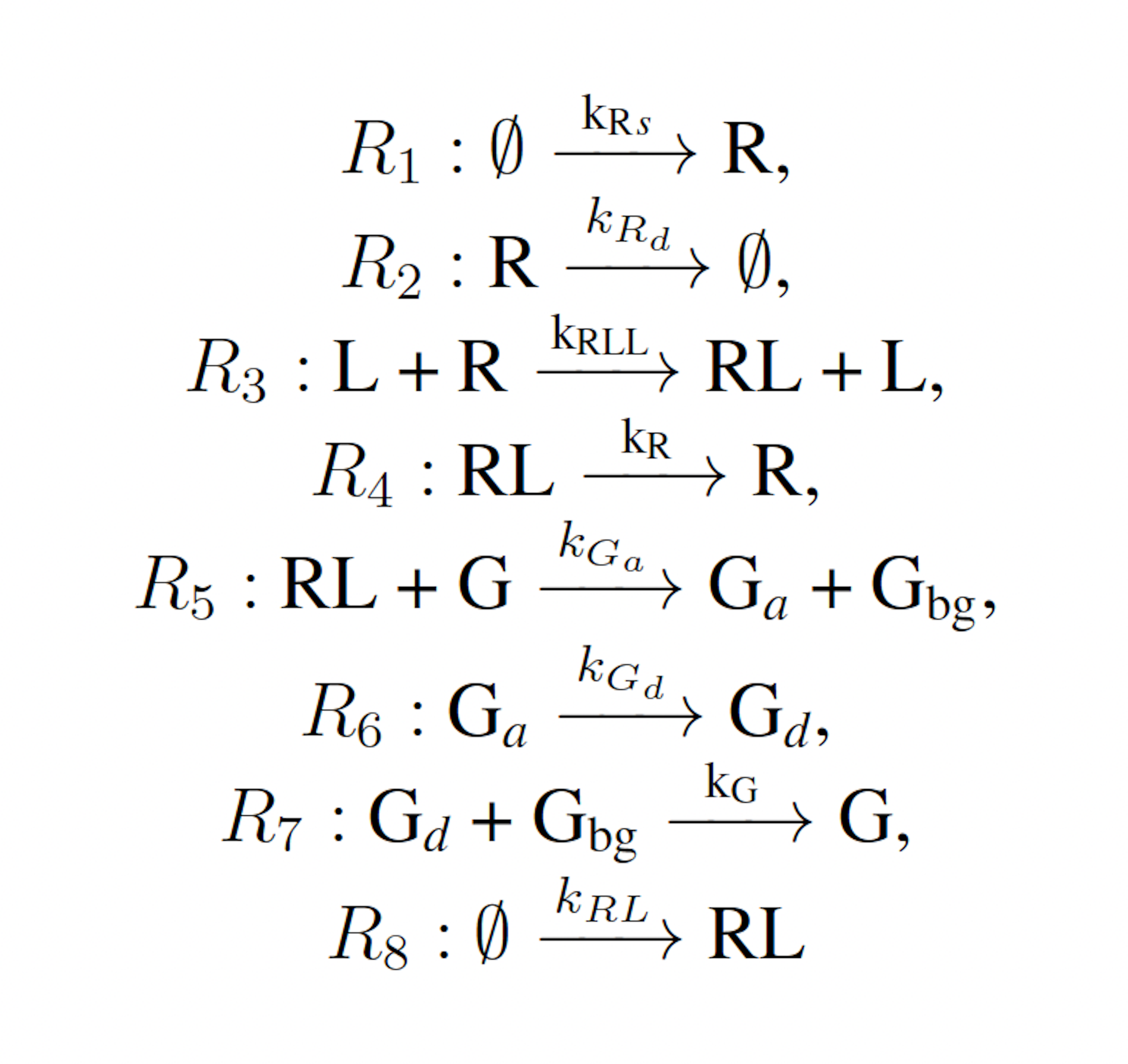
The modified yeast polarization model represents the pheromone induced G-protein cycle in Saccharomyces cerevisia [17]. This model is a more complicated naturally occurring biochemical reaction network than the futile cycle, and is given as follows:

where

The initial state of the model is set as follows:

This scheme yields the following analogous swSSA scheme:

3.1.3 Simplified Motility Regulation

The simplified motility regulation model represents the naturally occurring gene regulatory network which regulates flagella formation in Bacillus subtilis. This model serves as a an archetypal gene regulatory network, and is given as follows:

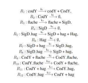
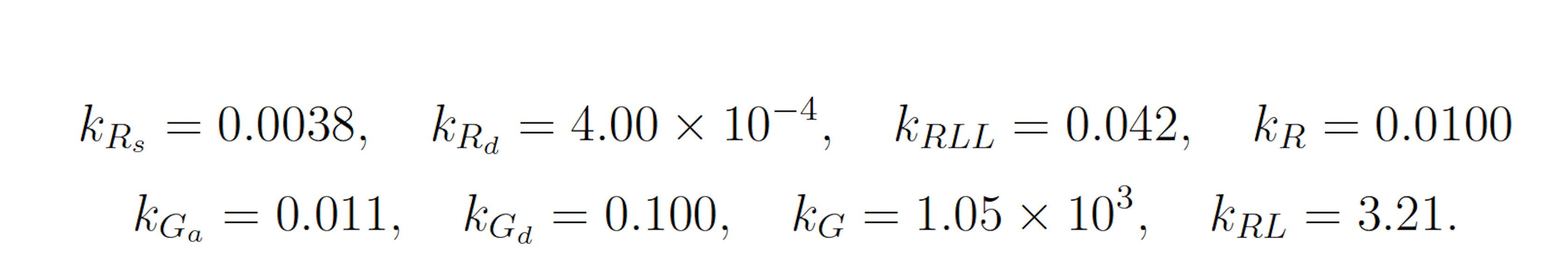
where

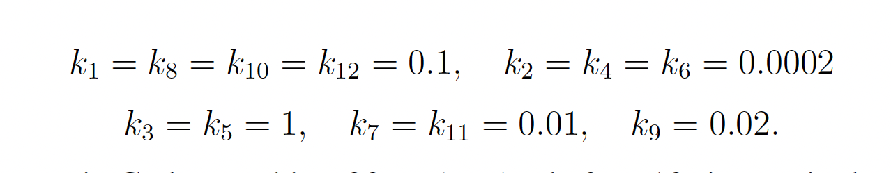
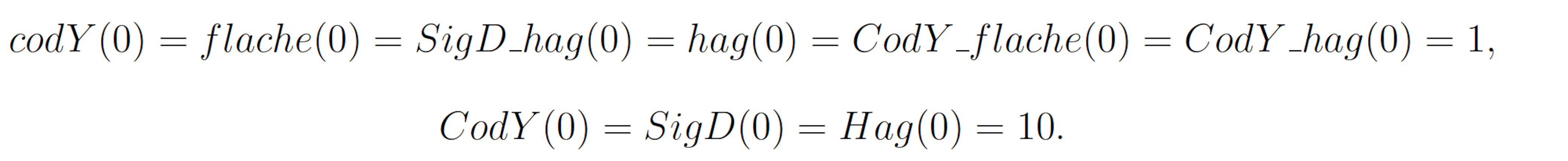
The rare event of interest is CodY reaching 20 molecules before 10 time units have passed. Subject to the following initial conditions:

The probability of this event has been previously calculated to be 2.161 × 10−7 [11]. We will consider this value to be exact. In the simplified motility regulation model, codY transcription/translation, Cod flache dissociation, and CodY hag dissociation may be increased and CodY degradation, CodY flache association, and CodY hag association may be decreased to increase the probability that CodY rises to 20. This gives the following wSSA weighting scheme:

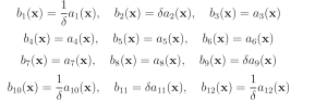
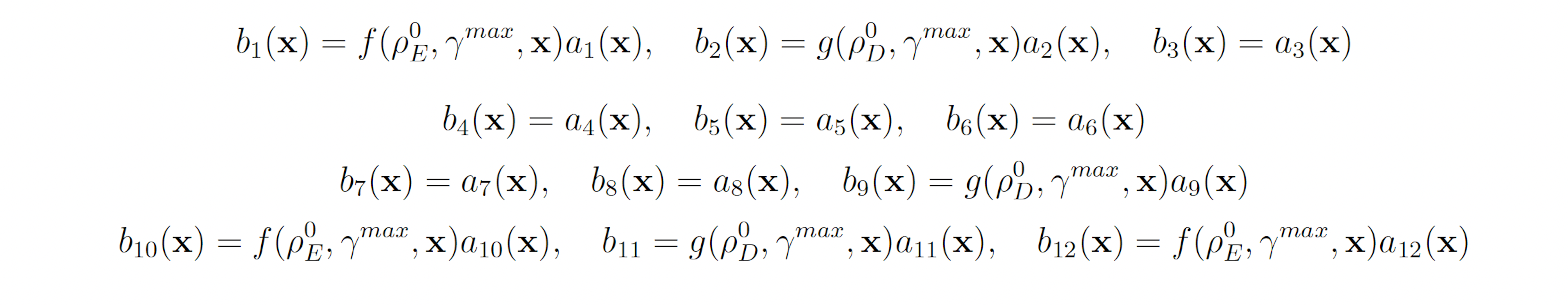
Again, we fix ρ0 D = 0.15 for all reactions selected to be biased downward and ρ0 E = 0.5 for all reactions selected to be biased upward. this gives the following swSSA weighting scheme:

3.1.4 Genetic Circuit 0x8E

Genetic circuit 0x8E is one of 60 genetic digital logic circuits designed using the genetic design automation tool Cello [15]. Circuit 0x8E has three input molecules Arabinose (Ara, ChEBI = 17535), Isopropyl-beta-Dthiogalactopyranoside (IPTG, ChEBI=61448) and Acetylcholine (aTc, ChEBI=15355), and one output, yellow fluorescent protein (YFP). This model serves as a archetypal genetic circuit. The input molecules have to be present for a prolonged time so that the input states can propagate through the different levels of logic. The circuit has three input molecules and therefore eight input combinations: (IPTG, aTc, Ara) ∈ {(0,0,0), (0,0,1), (0,1,0), (0,1,1), (1,0,0), (1,0,1), (1,1,0), (1,1,1)}, where one indicates the presence of a molecule and zero represents the absence of a molecule. Of these eight different input combinations, four result in the production of YFP and four do not. The circuit produces no YFP at steady state when (IPTG, aTc, Ara) = (1, 0, 0) or when (IPTG, aTc, Ara) = (1, 1, 1). However, if the circuit takes (IPTG, aTc, Ara) = (1, 0, 0) as an input and is then transitioned to (IPTG, aTc, Ara) = (1, 1, 1), YFP is transiently expressed before the circuit once again reacher steady state [4,5,15]. This unpredicted and unwanted behavior is known as a glitch. The genetic circuit 0x8E model consists of 15 reactions including 79 reaction rates. The rare event of interest is the quantification of that glitching behavior by determining the probability of YFP exceeding 70 molecules before 1000 time units pass. The probability of this event was estimated to be 6.29 × 10−4 with 106 runs of the SSA. We will consider this value to be exact. YFP production may be increased and YFP degradation may be decreased to increase the probability that YFP rises to 70. This gives the following wSSA weighting scheme:

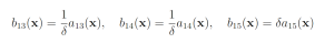
with all other reactions unbiased. Again fixing ρ0 D = 0.15 and ρ0 E = 0.5 gives the following swSSA weighting scheme:

3.1.5 Genetic Circuit 0x8E LHF

Genetic circuit 0x8E LHF is a Logic Hazard Free redesign of genetic circuit 0x8E [4]. The redesign utilized hazard-preserving optimizations to greatly reduce the glitching probability without changing the input molecules or stead state outputs of the original circuit 0x8E.

The model consists of 16 reactions including 94 reaction rates. The rare event of interest is the quantification of the glitching behavior by determining the probability of YFP exceeding 160 molecules before 1000 time units pass. The probability of this event was estimated to be 7.33 × 10−4 with 107 runs of the SSA. We will consider this value to be exact.

YFP production may be increased and YFP degradation may be decreased to increase the probability that YFP rises to 160. This gives the following wSSA weighting scheme:

3.1.6 Genetic Circuit 0x8E TI

Genetic Circuit 0x8E TI is a redesign of genetic circuit 0x8E with Two added Inverters to add extra delay to a pathway of the circuit to reduce its glitching behavior [4]. Like genetic circuit 0x8E LHF, genetic circuit 0x8E TI has reduced glitching probability compared to the original circuit 0x8E, but has the same inputs and output.

The genetic circuit 0x8E TI model consists of 19 reactions including 109 reaction rates. The rare event of interest is the quantification of the glitching behavior by determining the probability of YFP exceeding 100 molecules before 1000 time units pass. The probability of this event was estimated to be 8.74 × 10−4 with 107 runs of the SSA. We will consider this value to be exact.

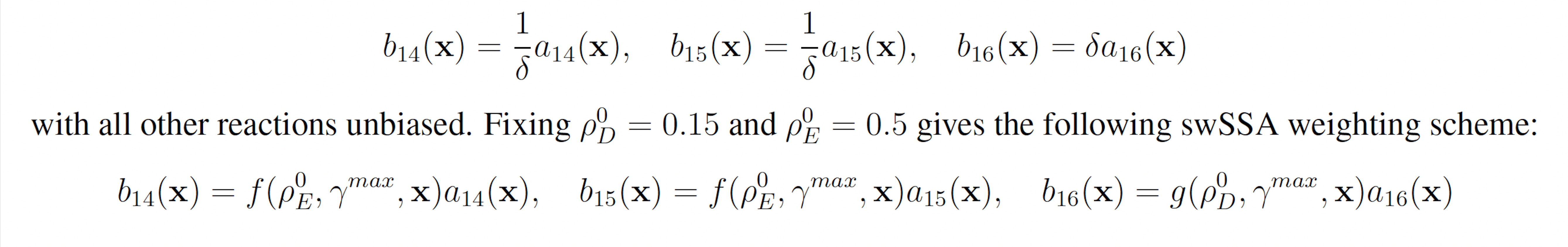
YFP production may be increased and YFP degradation may be decreased to increase the probability that YFP rises to 100. This gives the following wSSA weighting scheme:

3.2 Algorithmic Benchmarks

3.2.1 Biasing Parameter Optimization

For each model, we ran the wSSA with 30 values of δ from 0.05 to 1.5. Because the true probability of each rare event of interest is known, we may draw conclusions about which value(s) of δ performed most optimally for each model. The number of simulation runs was selected such that ’good’ and ’bad’ biasing parameters were easily discernible. We may also use these results to make claims about the robustness of each algorithm to biasing parameter variation. Similarly, for each model, we ran the swSSA an appropriate number of times with 33 values of γmax.The domain of these values was varied from model to model to attain optimal performance. As with the wSSA, we may draw conclusions about which value(s) of γmax performed most optimally and about the robustness of the swSSA.

3.2.2 Convergence Comparison

For each model, we performed 104 simulation runs with each algorithm. We selected this number of runs because it was sufficient for some but not all of the algorithms considered here to estimate the probability of the event of interest well in all models. After each simulation run, we calculated the estimated probability of the rare event of interest so that the rate of convergence of each algorithm could be visually compared. For these simulations, the wSSA and swSSA were given biasing parameters determined to be optimal.

3.2.3 Run Weight Variance Comparison

To compare the accuracy and precision of each method, we performed 103 simulation runs on each model. We then calculated the estimated probability of each model’s rare event of interest as well as the variance in the IS weight of simulation runs. Run weight variance has traditionally been used as a measure for biasing scheme optimality [9–11]. 3.2.4 Runtime Efficiency Comparison For each model, we performed 103 simulation runs for each algorithm and recorded the total run time (all simulation were performed on a machine with an Intel i7 4-core 2.11GHz processor and 8 GB of RAM, running Windows 10 Pro (v21H1)). This number of runs was selected because it yielded a run time on the order of seconds for most algorithms on most models. This revealed the run time efficiency of each algorithm as well as how that efficiency scales with model size.

3.2.3 Run Weight Variance Comparison

To compare the accuracy and precision of each method, we performed 103 simulation runs on each model. We then calculated the estimated probability of each model’s rare event of interest as well as the variance in the IS weight of simulation runs. Run weight variance has traditionally been used as a measure for biasing scheme optimality [9–11].

3.2.4 Runtime Efficiency Comparison

For each model, we performed 103 simulation runs for each algorithm and recorded the total run time (all simulation were performed on a machine with an Intel i7 4-core 2.11GHz processor and 8 GB of RAM, running Windows 10 Pro (v21H1)). This number of runs was selected because it yielded a run time on the order of seconds for most algorithms on most models. This revealed the run time efficiency of each algorithm as well as how that efficiency scales with model size.

4 Results

4.1 Enzymatic Futile Cycle

We first applied each importance sampling (IS) algorithm to the enzymatic futile cycle model (Section 3.1.1) to determine the probability of S5 falling to 25 molecules or fewer before 100 time units have passed. The enzymatic futile cycle is a typical biochemical motif, so these results are reflective of each algorithm’s ability to model rare events in simple biochemical systems. The probability of the event of interest in this model is p = 1.71 × 10−7.

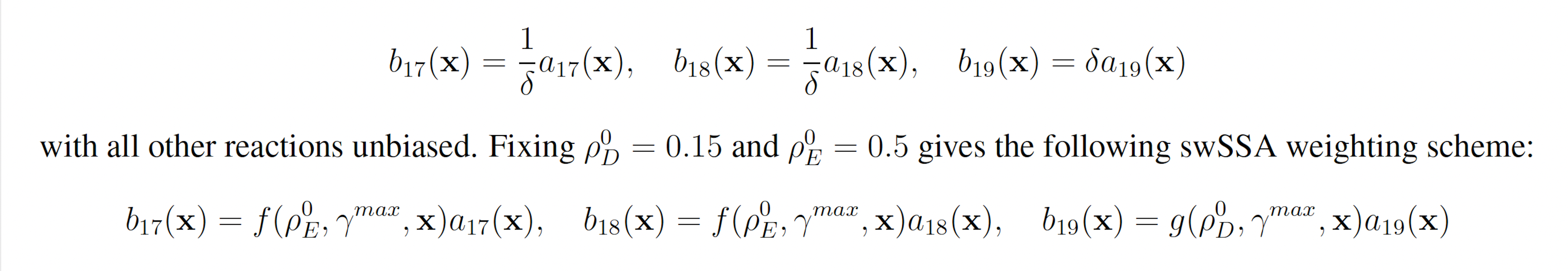
Figure 2: Simulation results for the enzymatic futile cycle model (true probability 1.71×10−7). (A) Convergence of Monte Carlo estimated probability for the SSA, wSSA, swSSA, and Guided wSSA over 104 runs (δ = 0.5, γmax = 2.5). (B) Probability estimated by the wSSA at 104 runs as a function of δ. (C) Probability estimated by the swSSA at 104 runs as a function of γmax. (D) Time for the SSA, wSSA, swSSA, and Guided wSSA to complete 103 runs.

We found that the wSSA and swSSA estimated p much faster than the SSA after 104 runs, but were sensitive to biasing parameters, while the Guided wSSA performed worse than the SSA. Biasing parameter optimization (Section 3.2.1) revealed that the wSSA and swSSA performed near optimally with biasing parameters δ = 0.5 and γmax = 2.5, respectively. However, both algorithms exhibited high relative error and poor performance as their biasing parameters varied from these values (Figure 2B and C). There is no existing technique for deriving these optimal biasing parameters without first knowing p. Convergence comparison (Section 3.2.2 revealed that, with these near-optimal biasing parameters, the wSSA and swSSA estimated p well within 104 runs, while the SSA and Guided wSSA failed to reach the state of interest even once (Figure 2A). The enhanced run efficiency of the wSSA and swSSA relative to the SSA does indicate that the user may estimate p more rapidly with these methods because the wSSA and swSSA performed with similar runtime efficiency (Section 3.2.4) to the SSA. The Guided wSSA, by contrast, was around 25% as efficient as the SSA despite performing similarly on this model (Figure 2D).

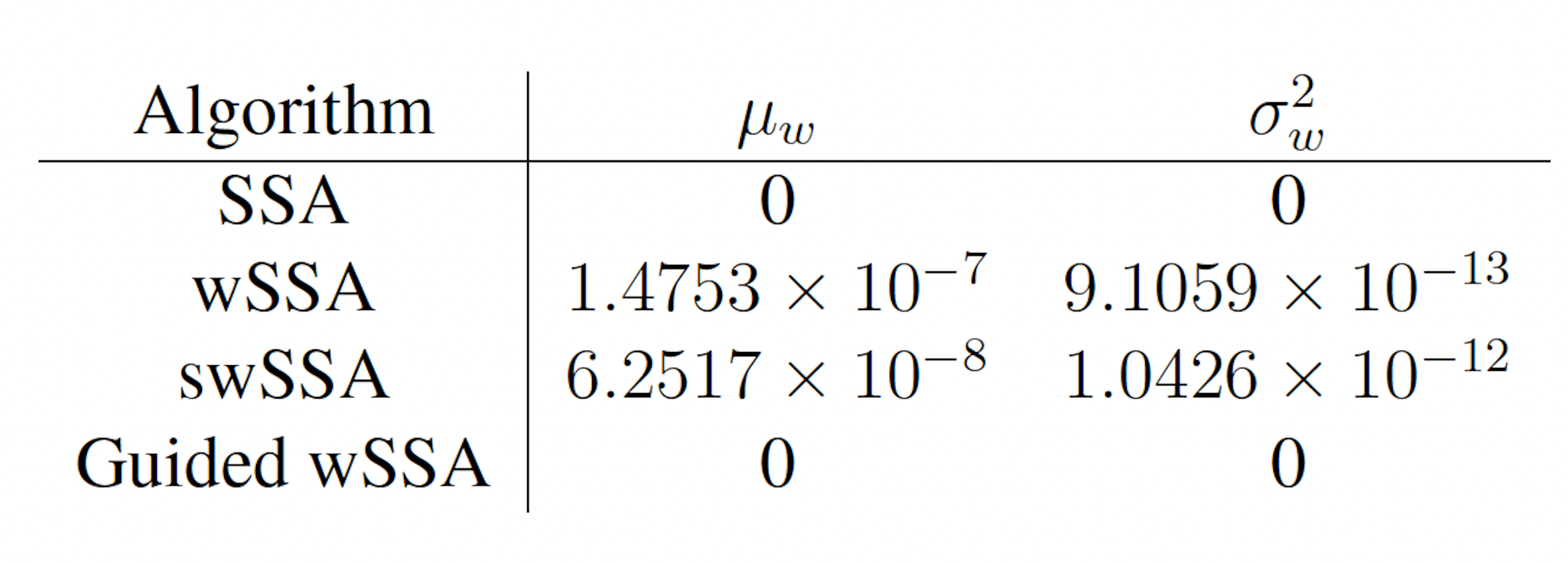
Table 1: Estimated probability and run weight variance produce by each algorithm when simulating the enzymatic futile cycle for 103 runs (true probability 1.71×10−7). Near-optimal biasing parameters were used for the wSSA and swSSA (δ = 0.5, γmax = 2.5).

We found that the wSSA estimated p more accurately and precisely than the swSSA. In 103 runs, the wSSA estimated p with 13.7% relative error while the swSSA estimated p with 63.4% relative error, indicating that the wSSA is more accurate. Likewise, the wSSA produced smaller run weight variance than the swSSA, indicating that the wSSA was also more precise. Given that the wSSA also performed with better runtime efficiency than the swSSA, it is clear that the state-dependent biasing applied by the swSSA was not helpful when simulating the enzymatic futile cycle (Table 1, Figure 2D).

4.2 Modified Yeast Polarization

Next, we applied each IS algorithm to the modified yeast polarization model (Section 3.1.2) to determine the probability of Gbg reaching 50 or more molecules before 20 time units have passed. The modified yeast polarization model is a typical biochemical reaction network which is more complicated than the enzymatic futile cycle, so these results are reflective of each algorithm’s ability to model rare events in more complicated biochemical systems. The probability of the event of interest in this model is p = 1.202 × 10−6.

We again found that the wSSA and swSSA estimated p much faster than the SSA after 104 runs, but were sensitive to biasing parameters, while the Guided wSSA performed worse than the SSA. Biasing parameter optimization (Section 3.2.1) revealed that the wSSA and swSSA performed near optimally with biasing parameters δ = 0.0.725 and γmax = 20, respectively. However, both algorithms exhibited high relative error and poor performance as their biasing parameters varied from these values (Figure 3B and C). There is no existing technique for deriving these optimal biasing parameters without first knowing p. Convergence comparison (Section 3.2.2 revealed that, with these near-optimal biasing parameters, the wSSA and swSSA estimated p well within 104 runs, while the SSA and Guided wSSA failed to reach the state of interest even once (Figure 3A). The enhanced run efficiency of the wSSA and swSSA relative to the SSA does indicate that the user may estimate p more rapidly with these methods because the wSSA and swSSA performed with similar runtime efficiency (Section 3.2.4) to the SSA. The Guided wSSA, by contrast, was around 33% as efficient as the SSA despite performing similarly on this model (Figure 3D). This disparity is less severe than in the futile cycle case, indicating that Guided wSSA was less slow relative to the other algorithms on this model.

We found that the swSSA estimated p more accurately and precisely than the swSSA, in contrast to the futile cycle case. In 103 runs, the wSSA estimated p with 3592.5% relative error while the swSSA estimated p with 0.3% relative error, indicating that the swSSA is more accurate. Likewise, the wSSA produced larger run weight variance than the swSSA, indicating that the swSSA was also more precise. In this case, it is clear that the statedependent biasing applied by the swSSA was helpful when simulating the enzymatic futile cycle. These results indicate that the superior performance of the wSSA in the futile cycle model does not generalize (Table 2).

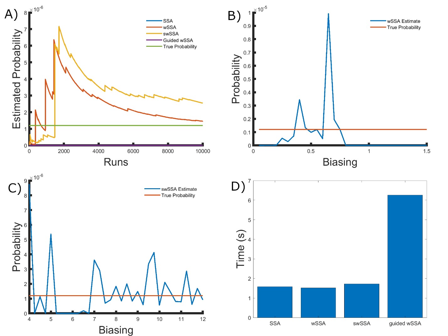
Figure 3: Simulation results for the modified yeast polarization model (true probability 1.202 × 10−6). (A) Convergence of Monte Carlo estimated probability for the SSA, wSSA, swSSA, and Guided wSSA over 104 runs (δ = 0.725, γmax = 20). (B) Probability estimated by the wSSA at 104 runs as a function of δ. (C) Probability estimated by the swSSA at 104 runs as a function of γmax. (D) Time for the SSA, wSSA, swSSA, and Guided wSSA to complete 103 runs.

4.3 Simplified Motility Regulation

Next, we applied each IS algorithm to the simplified motility regulation model (Section 3.1.3) to determine the probability of CodY reaching 20 or more molecules before 10 time units have passed. The simplified motility regulation model is a typical gene regulatory network, so these results are reflective of each algorithm’s ability to model rare events in naturally occurring gene regulatory networks. The probability of the event of interest in this model is p = 2.161 × 10−7.

We found that the wSSA, swSSA, and Guided wSSA estimated p much faster than the SSA after 104 runs, but the wSSA and swSSA were sensitive to biasing parameters. This is the first model in which the Guided wSSA outperforms the SSA. Biasing parameter optimization (Section 3.2.1) revealed that the wSSA and swSSA performed near optimally with biasing parameters δ = 0.3 and γmax = 8.25, respectively. However, both algorithms exhibited high relative error and poor performance as their biasing parameters varied from these values (Figure 4B and C). There is no existing technique for deriving these optimal biasing parameters without first knowing p. Convergence comparison (Section 3.2.2 revealed that, with these near-optimal biasing parameters, the wSSA and swSSA estimated p well within 104 runs, and the Guided wSSA did so without any user-selected biasing.

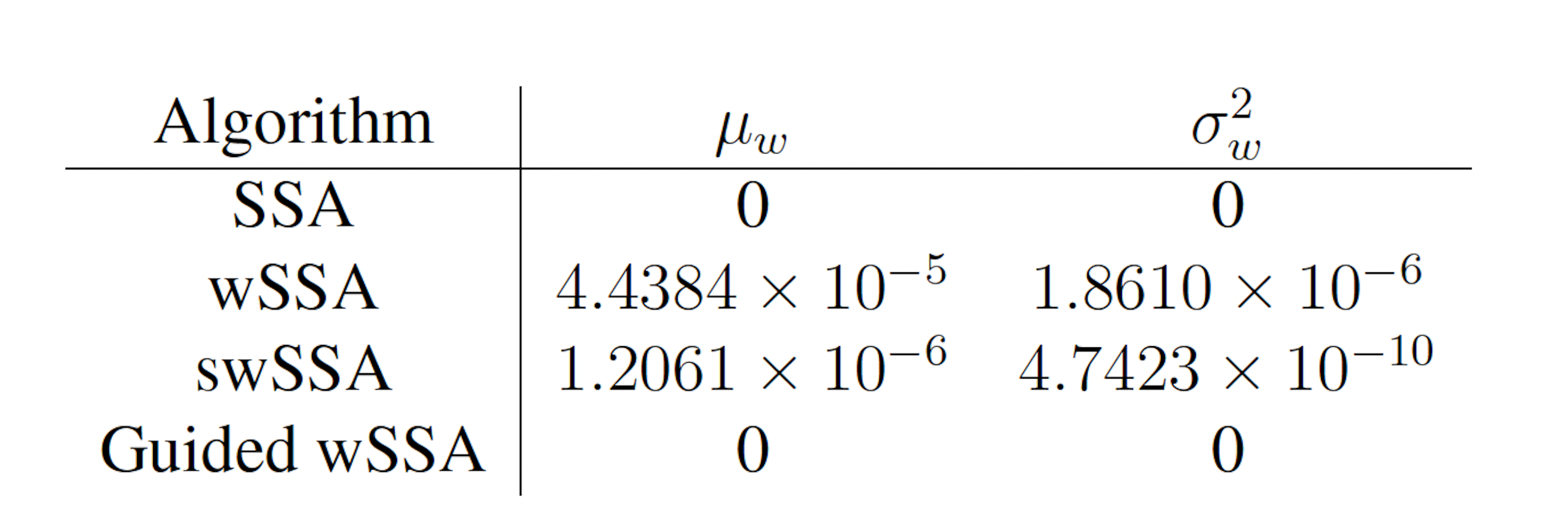
Table 2: Estimated probability and run weight variance produce by each algorithm when simulating the modified yeast polarization model for 103 runs (true probability 1.202×10−6). Near-optimal biasing parameters were used for the wSSA and swSSA (δ = 0.725, γmax = 20).

The SSA again failed to reach the state of interest even once (Figure 4A). The enhanced run efficiency of the wSSA and swSSA relative to the SSA does indicate that the user may estimate p more rapidly with these methods because the wSSA and swSSA performed with similar runtime efficiency (Section 3.2.4) to the SSA. The Guided wSSA was around 33% as efficient as the SSA but did perform well on this model (Figure 4D). In this case, the Guided wSSA is well-suited to the problem of rare event simulation and eliminates the need for biasing parameter selection.

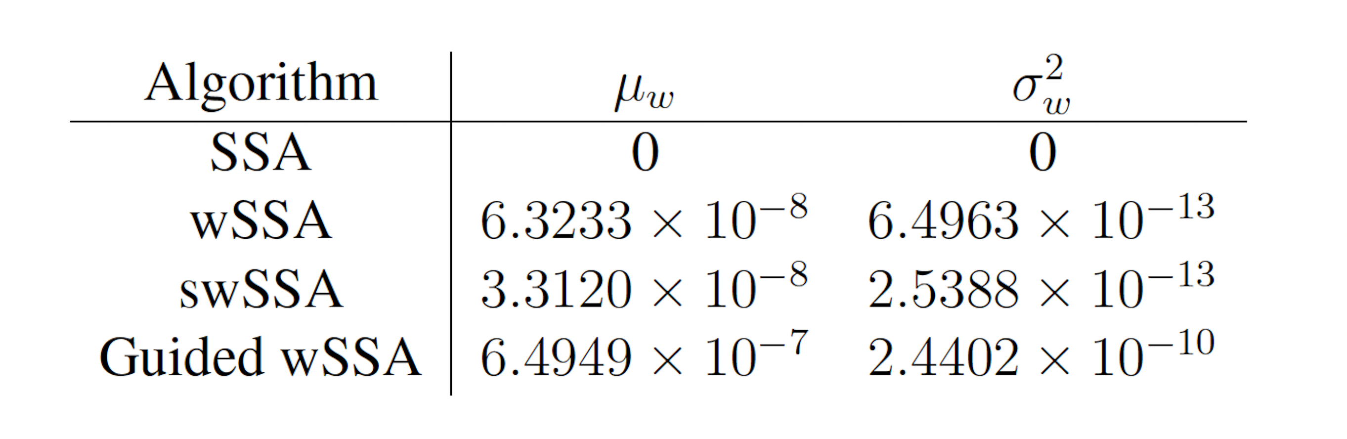
Table 3: Estimated probability and run weight variance produce by each algorithm when simulating the motility regulation model for 103 runs (true probability 2.161×10−7). Near-optimal biasing parameters were used for the wSSA and swSSA (δ = 0.3, γmax = 8.25).

We found that the wSSA estimated p more accurately and precisely than the swSSA or Guided wSSA. In 103 runs, the wSSA estimated p with 70.7% relative error while the swSSA estimated p with 84.7% relative error and the Guided wSSA estimated p with a 200.6% error, indicating that the wSSA is the most accurate. The Guided wSSA was also the least precise, though the swSSA was more precise than the wSSA despite being less accurate. This undermines the traditional use of run weight variance as a measure of IS scheme optimality. Though the wSSA and swSSA both performed better than the Guided wSSA in this case as they have in the previous two cases, the Guided wSSA does converge better than the SSA in this example. For this reason and because the Guided wSSA does not rely on user-selected biasing parameters, the Guided wSSA would be the safest option for this model, unlike in the previous two (Table 3).

4.4 Genetic Circuit 0x8E

Next, we applied each IS algorithm to the genetic circuit 0x8E model (Section 3.1.4) to determine the probability of Y FP reaching 70 or more molecules before 1000 time units have passed. The genetic circuit 0x8E model is a typical synthetic genetic circuit, so these results are reflective of each algorithm’s ability to model rare events in synthetic genetic circuits. The probability of the event of interest in this model is p = 6.29 × 10−4. We found that the SSA, wSSA, swSSA, and Guided wSSA all estimated p similarly after 104 runs, but the wSSA and swSSA were sensitive to biasing parameters and the Guided wSSA was inefficient. This is the first model in which the SSA performs well. Biasing parameter optimization (Section 3.2.1) revealed that the wSSA and swSSA performed near optimally with biasing parameters δ = 0.6 and γmax = 4.5, respectively. However, both algorithms exhibited high relative error and poor performance as their biasing parameters varied from these values (Figure 5B and C). There is no existing technique for deriving these optimal biasing parameters without first knowing p. Convergence comparison (Section 3.2.2 revealed that, with these near-optimal biasing parameters, the SSA, wSSA and swSSA, and Guided wSSA all estimated p well within 104 runs, and the SSA and Guided wSSA did so without any user-selected biasing (Figure 5A). The SSA is the best suited to rare event simulation in this case due to its lack of user-selected biasing parameters and superior runtime efficiency (Section 3.2.4, Figure 5D).

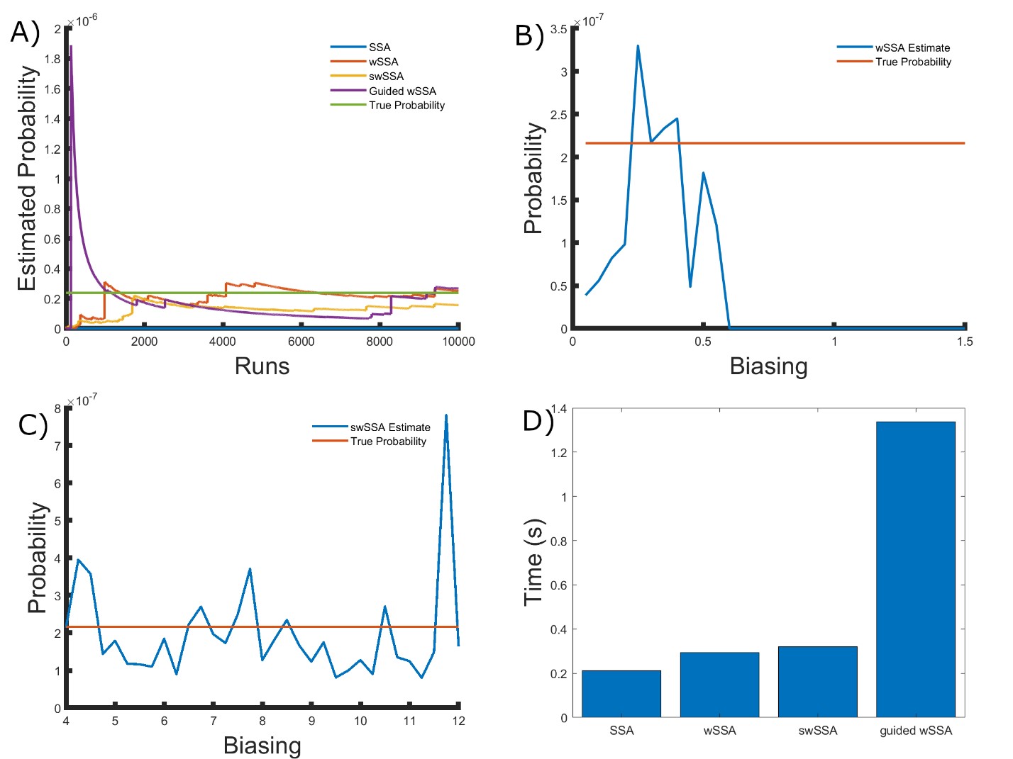
Figure 4: Simulation results for the simplified motility regulation model (true probability 2.161 × 10−7). (A) Convergence of Monte Carlo estimated probability for the SSA, wSSA, swSSA, and Guided wSSA over 104 runs (δ = 0.3, γmax = 8.25). (B) Probability estimated by the wSSA at 104 runs as a function of δ. (C) Probability estimated by the swSSA at 104 runs as a function of γmax. (D) Time for the SSA, wSSA, swSSA, and Guided wSSA to complete 103 runs.

the SSA, wSSA and swSSA, and Guided wSSA all estimated p well within 104 runs, and the SSA and Guided wSSA did so without any user-selected biasing (Figure 5A). The SSA is the best suited to rare event simulation in this case due to its lack of user-selected biasing parameters and superior runtime efficiency (Section 3.2.4, Figure 5D). We found that the wSSA estimated p more accurately and precisely than the SSA, swSSA or Guided wSSA. In 103 runs, the wSSA estimated p with 20.4% relative error while the swSSA estimated p with 56.6% relative error and the Guided wSSA estimated p with a 99.6% error, indicating that the wSSA is the most accurate. As in the modified motility regulation model, the Guided wSSA was also the least precise, though the swSSA was more precise than the wSSA despite being less accurate. This again undermines the traditional use of run weight variance as a measure of IS scheme optimality (Table 4).

4.5 Genetic Circuit 0x8E LHF

Next, we applied each IS algorithm to the genetic circuit 0x8E LHF model (Section 3.1.5) to determine the probability of Y FP reaching 160 or more molecules before 1000 time units have passed. The genetic circuit 0x8E LHF model is a typical synthetic genetic circuit like 0x8E, so these results are reflective of each algorithm’s ability to model rare events in synthetic genetic circuits. The probability of the event of interest in this model is p = 7.33 × 10−4.

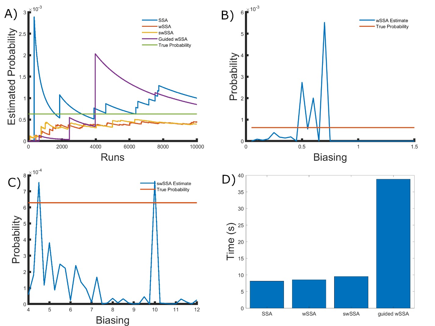
Figure 5: Simulation results for the genetic circuit 0x8E model (true probability 6.29 × 10−4). (A) Convergence of Monte Carlo estimated probability for the SSA, wSSA, swSSA, and Guided wSSA over 104 runs (δ = 0.6, γmax = 4.5). (B) Probability estimated by the wSSA at 102 runs as a function of δ. (C) Probability estimated by the swSSA at 102 runs as a function of γmax. (D) Time for the SSA, wSSA, swSSA, and Guided wSSA to complete 103 runs.

We found that the wSSA, swSSA, and Guided wSSA all estimated p similarly after 104 runs, but the wSSA and swSSA were sensitive to biasing parameters and the Guided wSSA was inefficient. Biasing parameter optimization (Section 3.2.1) revealed that the wSSA and swSSA performed near optimally with biasing parameters δ = 0.7 and γmax = 1.75, respectively. However, both algorithms exhibited high relative error and poor performance as their biasing parameters varied from these values (Figure 6B and C). There is no existing technique for deriving these optimal biasing parameters without first knowing p. Convergence comparison (Section 3.2.2 revealed that, with these near-optimal biasing parameters, the wSSA, swSSA, and Guided wSSA all estimated p well within 104 runs, and Guided wSSA did so without any user-selected biasing (Figure 6A). The Guided wSSA is the best suited to rare event simulation in this case due to its lack of user-selected biasing parameters, but is only around 33% as runtime efficient as the other methods (Section 3.2.4, Figure 6D). We found that the wSSA estimated p more accurately and precisely than the swSSA or Guided wSSA. In 103

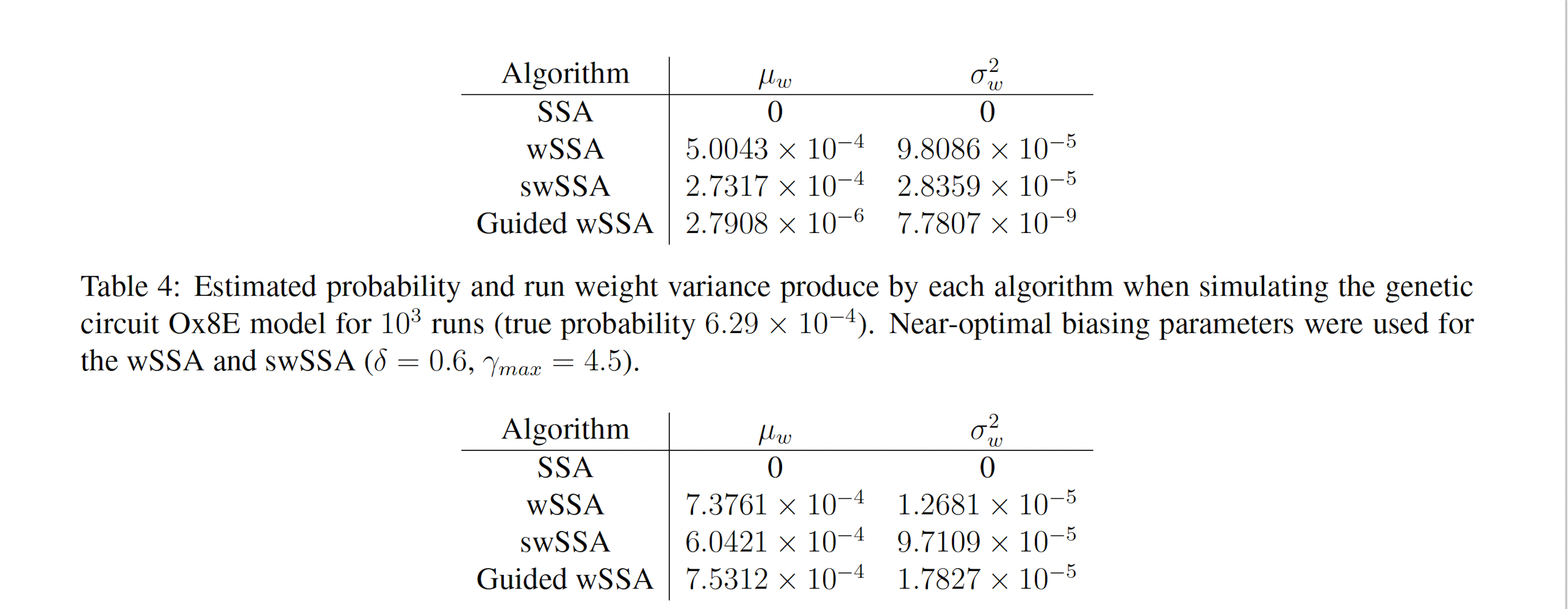
Table 5: Estimated probability and run weight variance produce by each algorithm when simulating the genetic circuit Ox8E LHF model for 103 runs (true probability 7.33×10−4). Near-optimal biasing parameters were used for the wSSA and swSSA (δ = 0.7, γmax = 1.75).

runs, the wSSA estimated p with 0.6% relative error while the swSSA estimated p with 17.6% relative error and the Guided wSSA estimated p with a 2.7% error, indicating that the wSSA is the most accurate. This is the first model in which the Guided wSSA outperformed the swSSA. In this case, low run weight variance was indicative of a superior performance (Table 5).

4.6 Genetic Circuit 0x8E TI

Next, we applied each IS algorithm to the genetic circuit 0x8E TI model (Section 3.1.6) to determine the probability of Y FP reaching 100 or more molecules before 1000 time units have passed. The genetic circuit 0x8E TI model is a typical synthetic genetic circuit like 0x8E and 0x8E LHF, so these results are reflective of each algorithm’s ability to model rare events in synthetic genetic circuits. The probability of the event of interest in this model is p = 8.74 × 10−4.

We found that the SSA and wSSA estimated p well after 104 runs, but the wSSA was sensitive to biasing parameters. This is the first model in which the swSSA does not perform well with optimal biasing parameters. Biasing parameter optimization (Section 3.2.1) revealed that the wSSA and swSSA performed near optimally with biasing parameters δ = 0.85 and γmax = 3.75, respectively. However, both algorithms exhibited high relative error and poor performance as their biasing parameters varied from these values (Figure 6B and C). There is no existing technique for deriving these optimal biasing parameters without first knowing p. Convergence comparison (Section 3.2.2 revealed that, with these near-optimal biasing parameters, the SSA and wSSA estimated p well within 104 runs, and the SSA did so without any user-selected biasing (Figure 7A). The SSA is the best suited to rare event simulation in this case due to its lack of user-selected biasing parameters and its superior runtime efficiency (Section 3.2.4, Figure 7D).

We found that the wSSA estimated p more accurately than the swSSA or Guided wSSA, though the swSSA and Guided wSSA reported higher precision. In 103 runs, the wSSA estimated p with 2.8% relative error while the swSSA estimated p with 85.2% relative error and the Guided wSSA estimated p with a 90.6% error, indicating that the wSSA is the most accurate. If the user were using run weight variance as a metric of optimality, they would fail to recognize the superior peroformance of the wSSA, however (Table 6).

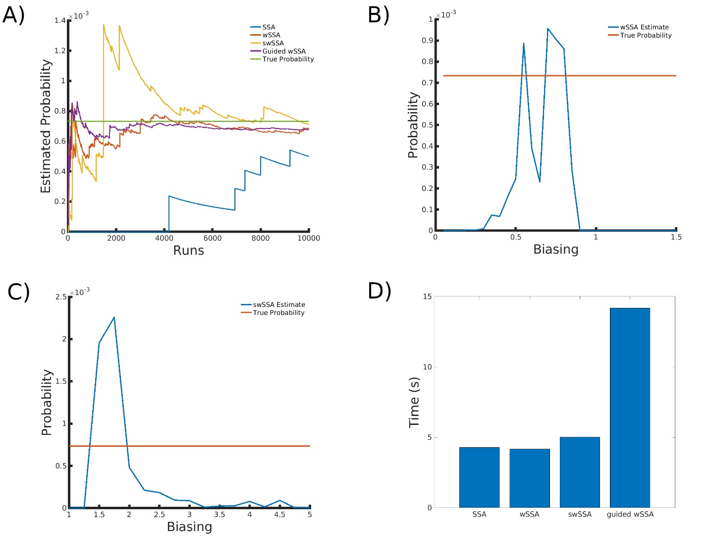
Figure 6: Simulation results for the genetic circuit 0x8E LHF model (true probability 7.33 × 10−4). (A) Convergence of Monte Carlo estimated probability for the SSA, wSSA, swSSA, and Guided wSSA over 104 runs (δ = 0.7, γmax = 1.75). (B) Probability estimated by the wSSA at 102 runs as a function of δ. (C) Probability estimated by the swSSA at 102 runs as a function of γmax. (D) Time for the SSA, wSSA, swSSA, and Guided wSSA to complete 103 runs.

4.7 Mathematical Analysis

We found that, across all our models, the wSSA and swSSA exhibited biasing parameter sensitivity and predominantly underestimated the true probability of the event of interest when given biasing parameters outside the narrow range of ’good’ parameters. Likewise, the Guided wSSA tended to underestimate the probability of the event of interest when it did not perform well. To understand why this occurs, we considered importance sampling schemes on a simple, abstract stochastic process.

Consider a process which being in state S0 and then transitions to some state in Ω = {S1, . . . , SN} with probability p1, . . . , pN, respectively. Denote this distribution as f. Let X be a random variable denoting the state the process enters after leaving S0 8. Suppose we want to know

p = P{X ∈ E}

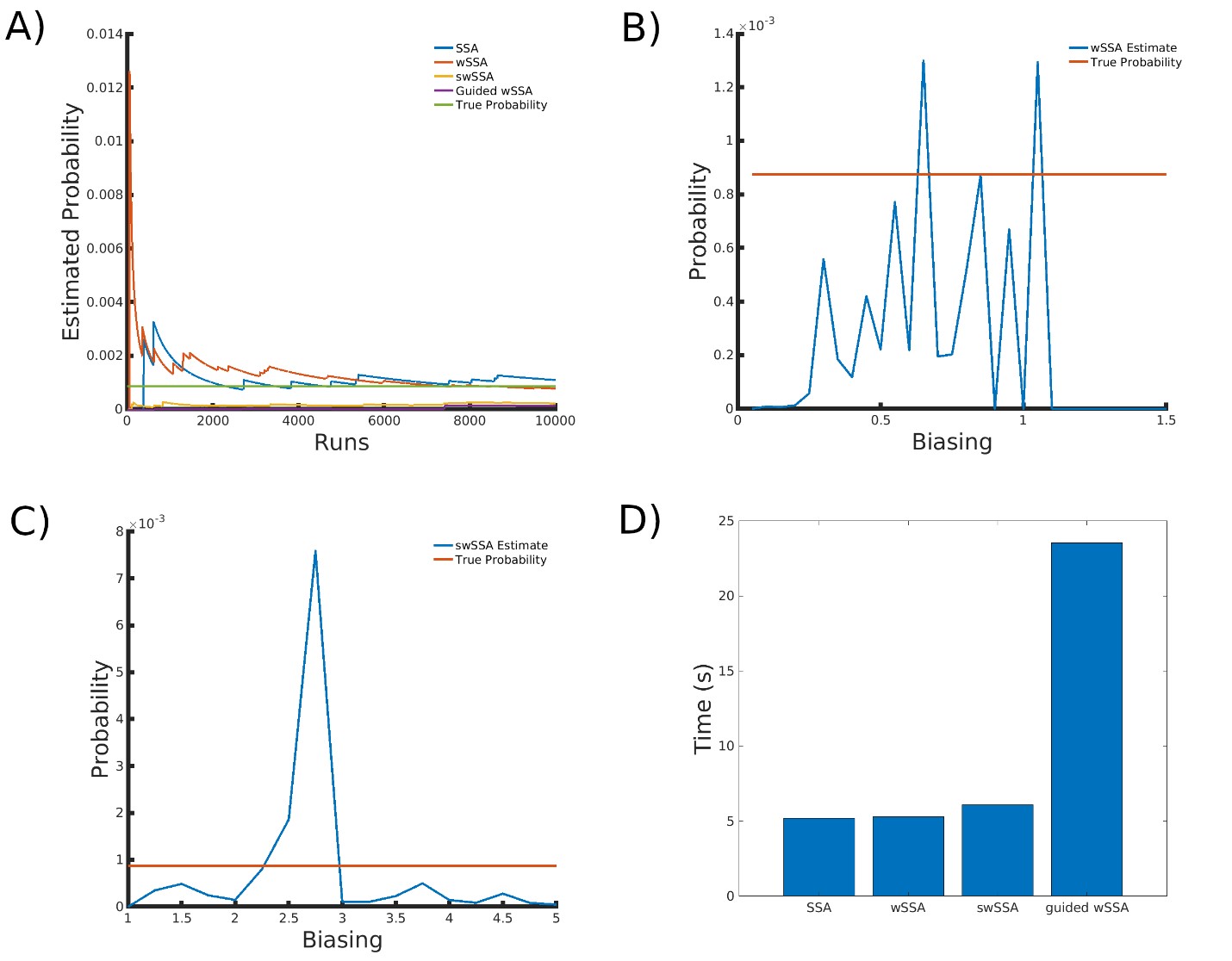
Figure 7: Simulation results for the genetic circuit 0x8E TI model (true probability 8.74×10−4). (A) Convergence of Monte Carlo estimated probability for the SSA, wSSA, swSSA, and Guided wSSA over 104 runs (δ = 0.85, γmax = 3.75). (B) Probability estimated by the wSSA at 103 runs as a function of δ. (C) Probability estimated by the swSSA at 103 runs as a function of γmax. (D) Time for the SSA, wSSA, swSSA, and Guided wSSA to complete 103 runs.

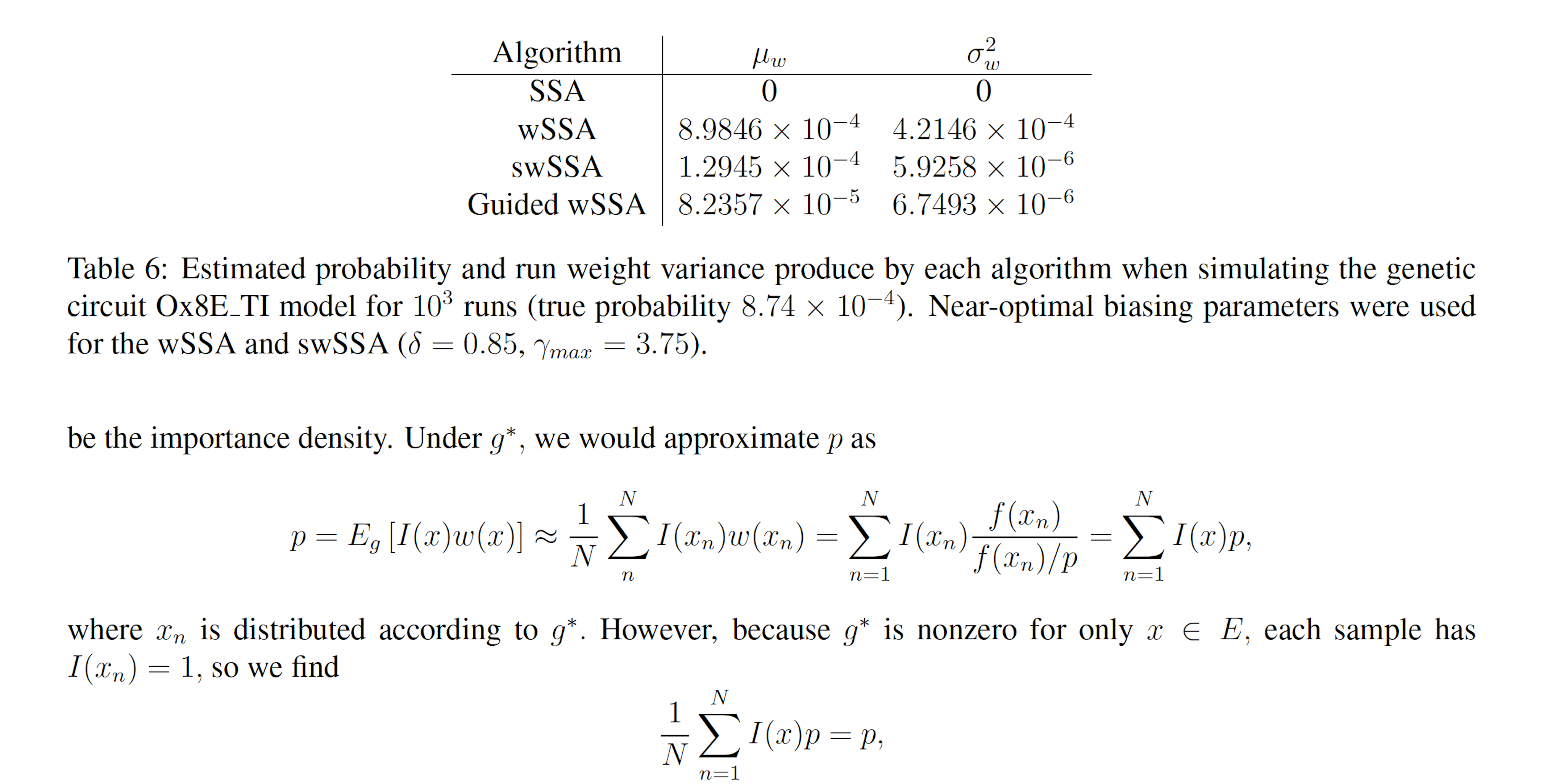
that is, the sample estimator under g∗ is always equivalent to p, so p may be exactly calculated with only one sample, and any set of samples with have a weight variance of zero. g∗ is therefore the ideal importance density [8]. Note that the ideal importance density is everywhere either zero or proportional to the distribution f. In practice, however, p is not known and it may be nonobvious which subset of the sample space E ⊂ Ω corresponds to a rare event of interest. Suppose instead we have the nonideal importance density.

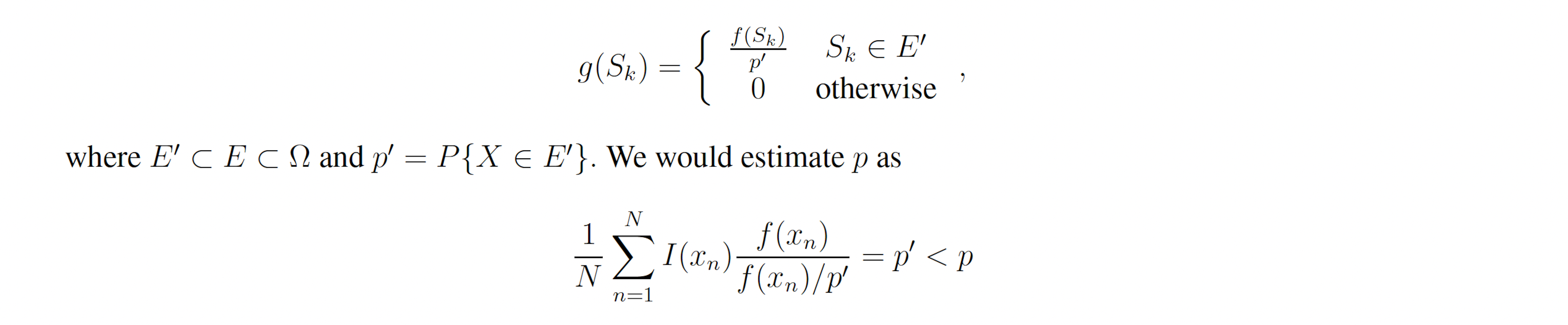
Note that, like the ideal importance density function g∗, the nonideal g yields zero-variance weights. In reality, a nonideal importance density may be vanishingly small but nonzero for x ∈ E −E′ and may slightly deviate from f(x)/p′ for x ∈ E′. In this case, many samples must be drawn from g before a single x ∈ E − E′ is produced. When one is, it will have a large weight because g(x) << f(x), which accounts for the exactness of importance sampling. However, before that sample is produced, the Monte Carlo estimator will yield an estimate very close to p′ with small weight variance. If small weight variance is used as an indicator of importance density optimality, such an importance sampling scheme will appear optimal while consistently producing underestimates for p. This issue is not a feature of rare event simulation, but rather a feature of importance sampling itself. It arises in the context of rare event simulation, however, because IS-based algorithms are not necessary when the events of interest are not rare. Within the context of the stochastic simulation algorithms for chemical reaction networks presented here, poor importance densities are sure to arise. This is because the methods considered here bias individual reactions, rather than individual elements of the sample space, that is, paths. Within this framework the importance density cannot be zero for paths which do not reach the state(s) of interest, nor can all paths to the state(s) of interest have importance density proportional to their true probability. In particular, the methods presented here bias some reactions upward and bias some downward. This causes paths to the state(s) of interest which include reactions which have been biased downward to have vanishingly small importance density, which leads to severe underestimates in all but the most optimal biasing schemes (Figures 2B-C, 3B-C, 4B-C, 5B-C, 6B-C, 7B-C). Likewise, the methods presented here produce large importance densities at paths which include many upward biased reactions but which do not reach the state of interest, which increases the number of zero-weight runs and delays estimator convergence further.

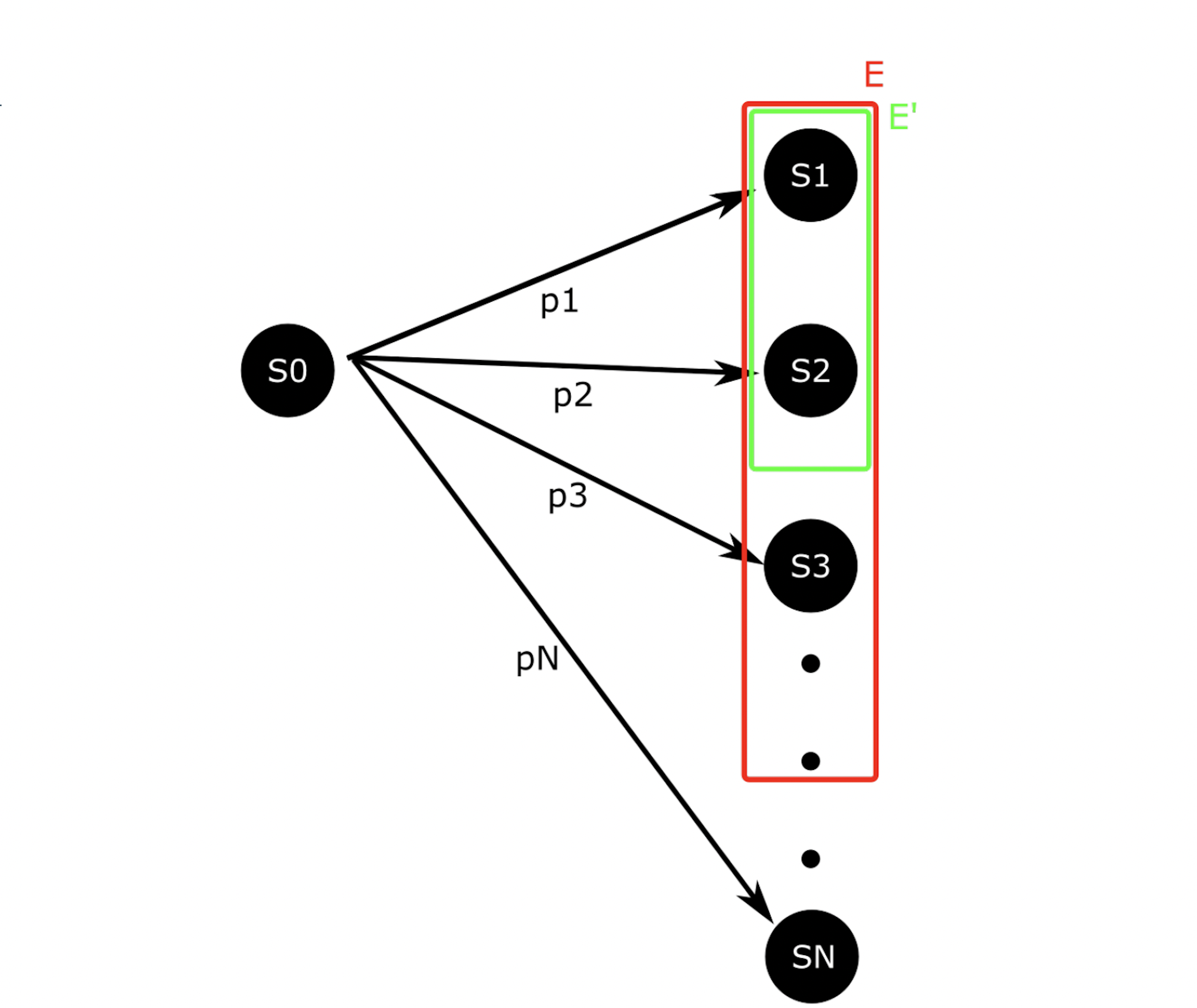
Figure 8: A simple, abstract stochastic process. Analysis of this process reveals the inherent challenges of ISbased algorithms.

5 Discussion

We implemented several existing stochastic simulation algorithms which make use of importance sampling (IS) to evaluate whether they were well-suited to the task of genetic circuit design verification. To this end, we developed a set of model biochemical systems case studies and algorithmic benchmarks which reflect the performance of an algorithmic in genetic circuit design. These analyses revealed that no existing algorithm is reliable enough to be used in design workflows. We concluded that IS-based simulation must be further developed to accelerate genetic circuit design.

Our investigations revealed that the weighted stochastic simulation algorithm (wSSA) [9] was able to estimate low probabilities more rapidly than any other method when given optimal biasing parameters (Figures 2A, 3A, 4A, 5A, 6A, 7A). The wSSA was able to do this as quickly or faster than the traditional SSA (Figures 2D, 3D, 4D, 5D, 6D, 7D). However, the wSSA also exhibited biasing sensitivity in all cases (Figures 2B, 3B, 4B, 5B, 6B, 7B). There does not exist any method for determining optimal biasing parameters without already knowing the true probability of the event of interest, as in our case studies. This makes the wSSA impractical for verifying actual genetic circuit designs. When the wSSA was biased poorly, it tended to underestimate the probability of the event of interest (Figures 2B, 3B, 4B, 5B, 6B, 7B), which is consistent with our understanding of IS methods in general (Section 4.7). Due to biasing sensitivity, the wSSA is not reliable enough to be used in genetic circuit design verification.

Likewise, the state-dependent weighted stochastic simulation algorithm (swSSA) [10] was able to rapidly estimate low probabilities (though not as rapidly as the wSSA) with optimal biasing parameters for all case studies (Figures 2A, 3A, 4A, 5A, 6A, 7A). The swSSA was able to do this with only a minimal loss of efficiency relative to the traditional SSA (Figures 2D, 3D, 4D, 5D, 6D, 7D). Again, however, the algorithm exhibited sensitivity to biasing parameters and there exists no method of determining which biasing parameters will be optimal without a priori knowledge of the event of interest (Figures 2C, 3C, 4C, 5C, 6C, 7C). The swSSA exhibited more robustness than the wSSA for smaller models (Figures 2C, 3C, 4C), but performed similar to the wSSA for actual genetic circuit designs (Figures 5C, 6C, 7C). The swSSA also underestimated probabilities when biased poorly, which is consistent with our understanding of IS methods in general (Section 4.7). Like the wSSA, the swSSA is too sensitive to biasing parameters to be used in genetic circuit design verification.

Unlike the wSSA and swSSA, the guided weighted stochastic simulation algorithm (Guided wSSA) [11] was not able to rapidly estimate the probability of rare events of interest in several of our case studies (Figures 2A, 3A, 7A). Despite its poor performance, the Guided wSSA also exhibited worse runtime efficiency than any other method, by a factor of around three (Figures 2D, 3D, 4D, 5D, 6D, 7D). The Guided wSSA does not rely on user-selected biasing parameters so it sidesteps the shortcomings of the wSSA and swSSA. However, the Guided wSSA is nonetheless too run-inefficient and time-inefficient to be suitable for genetic circuit design verification.

The wSSA, swSSA, and Guided wSSA each promised to solve the problem of rare event simulation in the verification of biochemical reaction networks in their respective publications [9–11]. We found this not to be the case. Previous work used run weight variance as a measure of biasing scheme optimality to show that IS methods perform well. However, we found that run weight variance is not suitable for that purpose (Tables 1, 2, 3, 4, 5, 6; Section 4.7). Additionally, The published description of the Guided wSSA is particularly misleading because modifications to the algorithm are required for it run stably and to replicated the published results (Section 2.3.3).

This work is limited, however, because each model was biasing using only one biasing factor, to simplify biasing factor optimization to a one-dimensional problem. The set of effective biasing schemes in higher dimensions may well vary in size and shape from the one-dimensional case. We also considered only individual simulation traces for each algorithm and model. A more robust approach would be to generate many traces and report on summary statistics instead.

Efficient and robust methods of rapidly estimating the probability of rare failure states are crucial to the computer aided verification of genetic circuits. If such methods can be developed, the design phase of the designbuild- test-learn (DBTL) cycle will be strengthened and genetic circuits will be prototyped much more quickly. To achieve this, however, more work is necessary. Future work may include the development of an IS-based stochastic simulation algorithm that is both run-efficient and time-efficient like the wSSA and swSSA but which is not reliant on user input like the Guided wSSA. Alternatively, future work could develop a method of deriving near-optimal biasing factors to be used with the wSSA or swSSA, perhaps using machine learning techniques. Future workflows could also make use of IS-based methods like those presented here to establish likely lower bounds on probabilities. Establishing a lower bound could prove useful if used in conjunction with other model checking techniques, such as counterexample generation [18].

Armed with efficient rare event simulation methods, synthetic biologists could make fewer orbits around the DBTL cycle when developing genetic circuits for applications in biofuels, biomanufacturing, and medicine. This would enable rapid prototyping of genetic devices which would have the potential to greatly improve quality of life.

6 Acknowledgements

We would like to thank the members of the Genetic Logic Lab at CU Boulder and the members of the Secure, Efficient, and Evolvable Computing Systems Lab at the University of South Florida, as well as the members of the FLUENT Verification Project at Utah State University, The University of Utah, and CU Boulder.

References

[1] Ahmad S. Khalil and James J. Collins. Synthetic biology: applications come of age. Nature Reviews Genetics, 11(5):367–379, May 2010.

[2] Rongming Liu, Marcelo C. Bassalo, Ramsey I. Zeitoun, and Ryan T. Gill. Genome scale engineering techniques for metabolic engineering. Metabolic Engineering, 32:143–154, 2015.

[3] Michael S Samoilov and Adam P Arkin. Deviant effects in molecular reaction pathways. Nature biotechnology, 24(10):1235–1240, 2006.

[4] Pedro Fontanarrosa, Hamid Doosthosseini, Amin Espah Borujeni, Yuval Dorfan, Christopher A. Voigt, and Chris Myers. Genetic circuit dynamics: Hazard and glitch analysis. ACS Synthetic Biology, 9(9):2324–2338, 2020. PMID: 32786351.

[5] Lukas Buecherl, Riley Roberts, Pedro Fontanarrosa, Payton J. Thomas, Jeanet Mante, Zhen Zhang, and Chris J. Myers. Stochastic hazard analysis of genetic circuits in ibiosim and stamina. ACS Synthetic Biology, 10(10):2532–2540, 2021. PMID: 34606710.

[6] Daniel T Gillespie. A general method for numerically simulating the stochastic time evolution of coupled chemical reactions. Journal of Computational Physics, 22(4):403–434, 1976.

[7] Daniel T. Gillespie. Exact stochastic simulation of coupled chemical reactions. The Journal of Physical Chemistry, 81(25):2340–2361, 1977.

[8] Surya T. Tokdar and Robert E. Kass. Importance sampling: a review. WIREs Computational Statistics, 2(1):54–60, December 2009.

[9] Hiroyuki Kuwahara and Ivan Mura. An efficient and exact stochastic simulation method to analyze rare events in biochemical systems. The Journal of chemical physics, 129(16):10B619, 2008.

[10] Min K Roh, Dan T Gillespie, and Linda R Petzold. State-dependent biasing method for importance sampling in the weighted stochastic simulation algorithm. The Journal of chemical physics, 133(17):174106, 2010.

[11] Colin S Gillespie and Andrew Golightly. Guided proposals for efficient weighted stochastic simulation. The Journal of chemical physics, 150(22):224103, 2019.

[12] Andrew Golightly and Darren JWilkinson. Bayesian inference for markov jump processes with informative observations. Statistical applications in genetics and molecular biology, 14(2):169–188, 2015.

[13] Timothy S. Gardner, Charles R. Cantor, and James J. Collins. Construction of a genetic toggle switch in escherichia coli. Nature, 403(6767):339–342, January 2000.

[14] Michael B. Elowitz and Stanislas Leibler. A synthetic oscillatory network of transcriptional regulators. Nature, 403(6767):335–338, January 2000.

[15] A. A. K. Nielsen, B. S. Der, J. Shin, P. Vaidyanathan, V. Paralanov, E. A. Strychalski, D. Ross, D. Densmore, and C. A. Voigt. Genetic circuit design automation. 352(6281). 26

[16] Ophir Flomenbom, Kelly Velonia, Davey Loos, Sadahiro Masuo, Mircea Cotlet, Yves Engelborghs, Johan Hofkens, Alan E Rowan, Roeland JM Nolte, Mark Van der Auweraer, et al. Stretched exponential decay and correlations in the catalytic activity of fluctuating single lipase molecules. Proceedings of the National Academy of Sciences, 102(7):2368–2372, 2005.

[17] Brian Drawert, Stefan Hellander, Michael Trogdon, Tau-Mu Yi, and Linda Petzold. A framework for discrete stochastic simulation on 3d moving boundary domains. The Journal of Chemical Physics, 145(18):184113, 2016.

[18] Mohammad Ahmadi, Zhen Zhang, Chris Myers, Chris Winstead, and Hao Zheng. Counterexample generation for infinite-state chemical reaction networks, 2022.