Science
107 CRISPR Perturbation of the Gene Regulatory Network That Specifies the Zebrafish Mesoderm
Tejashree Prakash
Faculty Mentor: James Gagnon (School of Biological Sciences, University of Utah)
ABSTRACT
During early development, zebrafish cells undergo gastrulation, a process that establishes a cell’s fate to develop mesoderm, a germ layer. Signaling pathways and key transcription factors (TFs) initialize a gene regulatory network that specifies and diversifies mesoderm during gastrulation. Three TFs – tbxta, tbx16, and noto – are essential for the mesodermal gene regulatory network, affecting initiation and maintenance of mesoderm derivatives such as the notochord and tailbud. tbxta, tbx16, and noto regulate one another through a series of additive and antagonistic interactions during different stages of gastrulation. My objectives are 1) to adapt a single-cell RNA sequencing (scRNA-seq) computational pipeline to characterize the molecular profiles of these three transcription factors, and 2) to understand the effects in cell types when these transcription factors are perturbed through CRISPR mutagenesis. Using a CRISPR mutagenesis to scRNA-seq pipeline, the mutant embryos are compared to the control embryos to analyze differences in gene expression and cell abundance. However, a challenge for using scRNA-seq data exists in defining shared cell types across samples. To address this problem, I have developed an agnostic computational framework to transfer previously established cell type labels onto a perturbed sample and analyze how gene expression and cell type abundances are affected. Cell type labels from reference atlases are the input for the annotation framework, which transfers these labels onto a perturbed dataset’s enriched cluster markers to identify its most likely cell types. By employing this framework, I identified the cell type changes across each perturbed condition in the developing embryos. My analysis recapitulates many known changes in cell abundance, such as loss of notochord and muscle, as well as novel changes in endoderm and aspects of ectoderm.
INTRODUCTION
Gastrulation is an essential process that defines the vertebrate body plan, possibly the most important event to occur in an organism’s lifetime. Gastrulation involves major cellular movements in a developing embryo, creating the first moment where stem cells commit to being progenitors for all cell types throughout the organism. Without this process, the cells of the embryo maintain pluripotency, where it is not confirmed to differentiate to a specific cell type. As the body of the embryo continues to develop, cells must obtain specific information as to what they will specify. This is the main purpose of gastrulation, to define the fate of cells in the embryo to commit to develop one of the three germ layers: ectoderm, endoderm, and mesoderm. In this overall process where a cell’s fate is established to develop one of the three germ layers, there are two primary events that occur. First, a cell’s fate is chosen to be ectoderm or mesendoderm; second, the mesendoderm cell’s fate is divided into mesoderm or endoderm, which goes on to make its corresponding germ layer’s derivatives.
The decision to induce mesendodermal cell types is defined by members of the Nodal signaling pathway (Campbell et al., 2005). Nodal signaling drives a pathway of receptor-transcription factor interactions that eventually regulates the expression of genes that are essential to developing the proper cell types in the appropriate regions of the embryo (Jones et al., 1995). Previous research has found that altering expression of Nodal signaling leads to large defects in mesendodermal regions. For example, experimental increasing of Nodal expression causes cells that normally develop for ectodermal cell types to reroute to mesendoderm. Transcription factors that are downstream effectors of Nodal signaling, such as cyc and sqt, are actively expressed even before the beginning of gastrulation, suggesting they are foundationally involved in defining embryonic regions of mesendodermal development (Campbell et al., 2005). Essentially, transcription factors that are controlled through Nodal signaling specify the location of specific mesendodermal cell types to belong to the margin, prechordal plate, etc., based on its intensity of expression. Those cell precursors then receive signals from mesendodermal genes to go on to develop structures such as the notochord, which is specific to the posterior axis of the embryo.
The mesodermal germ layer specifies muscle, bone, somites, and the circulatory and urogenital systems. At this point, the cell has its fate determined to develop mesoderm, through interactions involving Nodal signaling, and now the cell will express a combination of transcription factors that will guide its further development into mesodermal derivatives. For example, cells in the posterior axis of the embryo will receive Nodal signals to determine its mesoderm status, then a transcription factor like tbxta will be expressed in this region to guide the development of the notochord structure (Campbell et. al, 2005). These interactions between signaling pathways and transcription factors to finally establish a cell type is what is called a gene regulatory network. These interactions dictate the type and level of gene expression a cell experiences which in turn determines its function.
Three transcription factors, tbxta, tbx16, and noto, are known markers that guide the development and maintenance of mesodermal derivatives, acting as the mesodermal gene regulatory network. These three transcription factors have distinct but overlapping expression patterns in the mesodermal regions of the embryo. From previous research, tbxta and noto are known to be essential for development of the notochord, a cartilaginous spinal cord like structure along the dorsal side of the zebrafish. noto prevents the progenitor cells for notochord from differentiating as muscle cells (Campbell et al., 2005). In contrast, tbx16 is expressed in mesodermal cells to differentiate muscles and somites along the dorsal axis of the fish as well. tbx16 guides somite progenitors to the trunk of the fish, making it properly develop the corresponding somites of the trunk (Payumo et al, 2016). tbxta, tbx16, and noto have been studied for several years using different developmental biology and genetic techniques. Studies using techniques such as gene morpholinos have been used to study the function of these transcription factors by perturbing the gene of interest and seeing its phenotypic affects. tbxta mutants present a shortened or lack of tail; tbx16 mutants, also known as “spade tail”, fail to differentiate somite and muscle cells appropriately in the tail, leading to a knot-like form in the tail; and noto mutants display a lack of notochord and fused somites (Schulte-Merker et al., 1994; Payumo et al., 2016; Stemple et al., 1996). The interactions between these three transcription factors remain unclear, whether they work synergistically, antagonistically, or perhaps a combination of the two. Thus, I study these three transcription factors using a set of novel tools to provide a different, molecular perspective of how these transcription factors interact to specify different layers of mesoderm.
Novel tools to study genetics and developmental biology have become more accessible to researchers, allowing classic developmental questions to be questioned in new perspectives. The CRISPR/Cas9 system is a gene editing technique that can introduce precise edits in an endogenous genomic locus of an organism (Ran et al., 2013). This genome editing method can be equipped in gene perturbation screenings, which is how it is applied in my experiment. Cas9 enzyme targets a site in the genome of the zebrafish complementing a guide RNA uniquely designed for the gene target of interest. The Cas9 then induces a double stranded break and excises this target sequence. The removal of the target sequence ultimately induces a permanent mutation at that genomic site, causing a loss of function phenotype in the mutant embryo. CRISPR/Cas9 provides a new and relatively simpler method for genetic engineering that I have applied to study the mesodermal gene regulatory network through the induction of transcription factor perturbations.
Single-cell RNA sequencing (scRNA-seq) is a technology that enables the measurement of RNA transcripts from individual cells of an embryo, permitting analysis of the molecular compositions of each cell. In this method, mutant embryos of interest, acquired through CRISPR mutagenesis in my project, are dissociated into a state of single cell suspension, and submitted for 10X Genomics for scRNA-seq. The 10X Genomics method for scRNA-seq pools gel beads containing individual barcodes with each sample of single cells. A reaction takes place where the beads dissolve to tag mRNAs from each single cell with a unique barcode. These barcoded fragments are then assembled to generate a sequencing library for each mutant embryo. This constructed sequencing library maps each RNA read to its corresponding single cell, meaning that the library displays individual cell with its attributed molecular composition. The library is aligned to the zebrafish transcriptome of choice and put through a series of analysis pipelines in R to determine shared cell populations across conditions, determining relative levels of cell abundance and gene expression. The combination of CRISPR/Cas9 technology with scRNA-seq provides avenues to understand the function of transcription factors through the perspective of cell abundance and gene expression, which is why I employ these technologies to study the mesodermal gene regulatory network.
Single-cell profiles require further manipulation to yield comprehensible information regarding the cell type composition of a given sample. As the output of single-cell sequencing experiments, single-cell datasets only maintain an identification of what sample condition each cell belongs to and what genes compose that cell, but not its specific cell type label. Previous genetic studies have compiled what genetic markers make up a particular cell type, but these datasets are not necessarily translatable to single-cell datasets in an automatic method. This creates a challenge in defining shared cell types across multiple perturbed samples efficiently, as manually doing so is time consuming and may lead to inaccurate labels. Therefore, I have created and applied an agnostic computational method that will transfer labels onto a perturbed single-cell dataset based on its composition of shared genetic markers. The ability to label cell types will identify what cell type the differences in cell abundance belong to, filling in that last space to have comprehensible molecular composition information for single cells. Ultimately, the combination of the optimized CRISPR/scRNA-seq method with my computational framework will provide hypotheses for what cell type interactions are taking place when mesoderm cell types are perturbed in zebrafish embryos.
METHODS
Generation of gRNAs
Three gRNA sites were developed for each transcription factor, tbxta, tbx16, noto, and tyr by choosing target sites with high efficiencies and no overlap with one another on CHOPCHOP.
CRISPR/Cas9 Microinjection Mix
CRISPR injection mixes for tbx16, noto, and tyr were assembled with its corresponding gRNA in the following order: 1.5 µl 1M KCl (Sigma-Aldrich), 1.5 µl of the corresponding gRNAs, as generated above, 0.5 µl of phenol red (Sigma-Aldrich), and 1.5 µl of 20 µM CRISPR protein (Engen). The injection mix to target tbxta was assembled in an identical manner, except 1.0 µl of tbxta gRNA and 0.5 µl of pure H2O was used. The injection mixes were vortexed briefly to ensure proper mixing and kept on ice until used for embryo microinjection. During initial microinjection experiments, the tbxta injection mix was seen to have greater instances of cell death and toxicity. 3-4 puffs of injection mix were used, once the needle was calibrated, for tbx16 and noto, and 2-3 puffs were used for tbxta.
Embryo Dissociation
Embryos were allowed to develop to 24 hours post injection, and those displaying a strong phenotype were chosen and placed in 1.5 ml Eppendorf tubes for dissociation and sequencing. The embryos were first dechorionated. Egg water was removed from each tube of embryos and replaced with 1 ml of 1mg/ml Pronase in 0.3X Danieau Buffer. The tubes were swirled gently for 3 minutes, and the Pronase solution was replaced with 1mL of 0.3X Danieau Buffer. This process of washing with Pronase then Danieau Buffer was repeated at least 4 times, until the chorions fell apart for all embryos. Once the embryos were dechorionated, the dissociation protocol was applied. The Danieau Buffer from the last dechorionation wash was replaced with 1mL of FACSmax solution. The tubes were triturated to homogeneity by pipetting up and down with p1000 pipette, until the tissue was properly broken up. Adding additional FACSmax solution, the tubes were incubated at 28°C for 20 minutes, pipetting every 10 minutes to break up tissue. The solutions containing the embryos were passed through a 40um cell strainer to a new 50 ml Falcon tube. The cell pellets were centrifuged at 310 x g for 5 minutes, then the supernatant was discarded and replaced with 1 mL of PBS. The tubes were centrifuged additionally at 310 x g for 5 minutes, with the cell pellets resuspended in 1X PBS diluted with 0.5% BSA. The tubes of dissociated embryos were kept on ice and submitted for 10X single-cell RNA sequencing.
PCR / Gel Electrophoresis
The genomic DNA was first extracted from the four mutant conditions through the “HotShot” DNA preparation method. First, egg water was pipetted out and replaced of 50 ul of Alkyl Lyse, incubated at 95°C for one hour using a thermocycler, and 50 ul of Neutralizer was lastly added. Alkyl Lyse was developed with 25mM NaOH and 0.2mM EDTA, and the Neutralizer reagent was 40mM Tris-HCl. Aliquots of the primers for each TF were then made, consisting of 10uM of the stock primer previously developed for each TF’s gRNA sequence. The PCR mix was created for each condition to a total volume of 25 ul: 1.25 ul reverse primer and 1.25 ul of forward primer, 3 ul of genomic DNA, 7 ul of pure H2O, and 12.5 ul of Q5 reagent. Along with the mutant genomic data, wildtype embryos were combined with each primer combination to allow for control analysis. The genomic data that has now been amplified were stained with 5ul of loading dye and loaded into a gel electrophoresis, along with the DNA ladder, in 120V for 25 minutes. A 1% agarose gel was created for the gel electrophoresis.
Single-Cell Data Import – Cell Ranger
The single-cell data retrieved from scRNA-seq submissions were aligned to the Lawson zebrafish transcriptome through Cell Ranger analysis pipelines (Lawson et al, 2020). Each raw single-cell dataset’s reads were appropriately mapped to the transcribed regions of the zebrafish genome through what was defined within the Lawson transcriptome. Cell Ranger ultimately outputs two files for each single-cell dataset: the “filtered_features_bc_matrix” with the mapped RNA reads and an html document summarizing the features of the dataset, such as cell count, number of reads, percent of reads mapped to genome, etc. The filtered_features_bc_matrix file for each sample, containing the barcodes, features, and matrix files, was the foundational data used in the Satija Lab’s Seurat computational pipelines.
Single-Cell Data Analysis – Seurat Protocols
Cell Clustering
The “Guided Clustering Tutorial” from Seurat was applied to define clusters, or groups of cell populations, for the single-cell data of each perturbed condition (Hoffman, 2023a). Beginning with a Seurat object containing the “filtered_features_bc_matrix” file from Cell Ranger, the initial single-cell analysis requires a series of quality control (QC), filtering, and normalization methods. QC metrics, removing unwanted cells, were visualized through violin plots, where the cells are filtered to only include unique feature counts over 2,500. The data was then normalized, and a visualization determining the highly variable features was created using the FindVariableFeatures function. The highly variable features of a dataset are defined as features highly expressed in some cells while lowly expressed in others, important for further downstream analyses. Linear dimensional reduction (RunPCA function) was performed, where these PCA scores determine the principle components in a variable feature set so like cells are clustered together. The function for creating clusters is FindClusters. The final step in this tutorial was applied to the single-cell datasets to visualize the clusters previously determined. UMAP, a non-linear dimensional reduction technique, colocalizes like cells, belonging to its cluster, together in a low-dimensional space.
Multiple Single-cell Dataset Integration
Seurat’s “Introduction to scRNA-seq Integration Tutorial” was applied to integrate the perturbed conditions into one dataset (Hoffman, 2023b). The purpose of the integration was to create a new object that contained shared cell populations across multiple sample conditions. The integrated object creates ease in future analyses to identify differences in shared cell types across the different perturbed conditions. To achieve this, pairs of cells were identified across the multiple datasets that share the same biological state, or cell type, using the FindIntegrationAnchors function. These pairs of cells acted as the anchor points for congregating all the different sample’s cluster data into a single dimensioned object, through the IntegrateData function. The now integrated object was put through a standard workflow for re-clustering and finally visualized as a UMAP plot. The FindNeighbors function specified what number of clusters the dataset should be forced to; the dimension yielding 45 clusters, unique to the integrated object, was used. Individual perturbed conditions were finally visualized in the integrated UMAP plot by using the split.by function, allowing differences in cell abundance between perturbed conditions to be visualized.
Label Transfer Computational Method
My code for these analyses are available at: https://github.com/Gagnon-lab/label-transfer-method
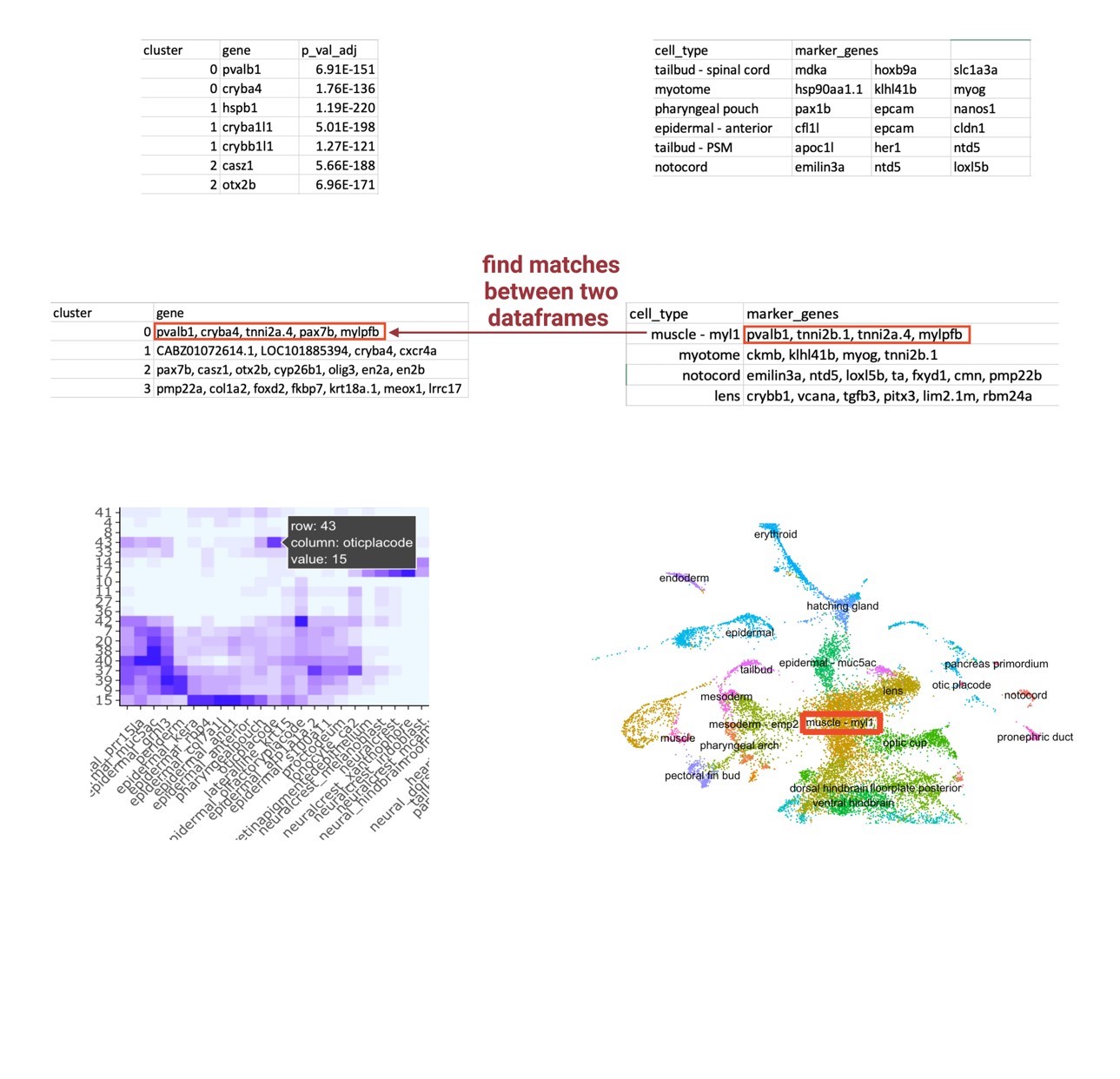
The integrated object determined cell populations shared across the different perturbed conditions but did not automatically allow those populations to be identified. The label transfer method was developed and applied to label these clusters using a previously established reference cell atlas that has defined the top markers expressed for a cell type. The first input for this computational method was the highly differentiated markers expressed for each cluster of the integrated object, obtained through the FindAllMarkers function in Seurat and filtered to only contain the genes that have a p value significance of less than 0.05. The second input was the Wagner Lab’s reference cell atlas that defines the top 20 markers that defines a cell type for the 24hpf developmental stage (Wagner et al., 2018). Each input was formatted to be a compatible data frame, making a list of markers that defines each cell type of the cell atlas and each unlabeled cluster from the FindAllMarkers output. These two data frames were then compared to each other to create a match vector containing the magnitude of genes in common as well as a list of those genes. Ultimately, the highest match vector between a certain cell type and unlabeled cluster comparison will attribute that cell type to that cluster. The final outputs of the label transfer method were a heatmap displaying the magnitude of matches between the cell type reference and the cluster information as well as a table summarizing the highest match vectors; therefore, the label transfer method works to predict what the most likely cell type identification each previously unlabeled cluster is. The label transfer method has been adapted to a function in R called label_transfer. The function requires three inputs as .csv files: “annotation”, “clusters”, and “cell_type_names”. “Annotation” is the reference cell atlas of choice as a data frame, “clusters” is the FindAllMarkers output as a data frame, and “cell_type_names” is a data frame with only the name columns of the reference cell atlas. The label_transfer function outputs the heatmap and table summarizing cluster-cell type matches, as previously described.
Calculating Differences in Cell Abundance
Cluster-by-cluster, cell counts in each condition were logarithmically compared to the control condition, the tyr-injected condition. This was done by splitting up the integrated object condition-by-condition, and a log10 transformation calculation was done to create logarithmic comparisons. A data frame consisting of these comparisons was developed, positive values for increases in cell abundance compared to the control and negative values for decreases in cell abundance compared to the control. This data frame was employed to create a heatmap, using melt and ggplot R packages, to visualize the cell abundance changes, with the scale being a logarithmic scale of -1 to 1, with 0 being no change. Each cluster has an identity attributed to it through the previous label transfer method.
RESULTS
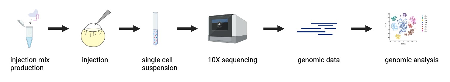
| Figure 1: CRISPR Mutagenesis to Single-Cell RNA Sequencing Pipeline. An objective of this project was to optimize the pipeline of inducing CRISPR-mediated mutants in zebrafish embryos to obtaining single-cell RNA sequencing genomic data, and apply it to study the mesodermal gene regulatory network. |
As previously stated, tbxta, tbx16, and noto are transcription factors (TFs) that initialize a gene regulatory network that specifies and diversifies mesoderm during gastrulation. The overarching objective of my project was to explore how these factors work together and individually to make different layers of mesoderm through the use of new developmental biology tools. I developed a CRISPR mutagenesis to scRNA-seq pipeline to study the function of these three TFs, as shown in Figure 1. My project can be summarized into a few steps: generation of mutants, dissociation to single cells and submission to 10X single-cell RNA sequencing, and the analysis of the scRNA-seq data. Perturbations were generated for tbxta, tbx16, and noto using a CRISPR-Cas9 system optimized to obtain mutants that recapitulate the TF’s known mutant phenotypes. These embryos were dissociated into single cells and submitted for 10X single-cell RNA sequencing, yielding single-cell profiles of each mutant embryo condition for computational analysis.
- Generation of Mutants
The first objective was to generate embryos for each condition, with tyr-injected embryos acting as a control experiment, as this gene only targets the pigmentation of the fish without influencing mesoderm or other cell types during development. These mutant embryos were generated for each condition using the CRISPR-Cas9 system. The CRISPR-Cas9 system uses an injection mix with pooled gRNAs that targeted each gene of interest with the CRISPR protein to essentially cause loss-of-function mutations for each condition (Figure 2a). The gRNAs I designed for each TF were chosen through CHOPCHOP.
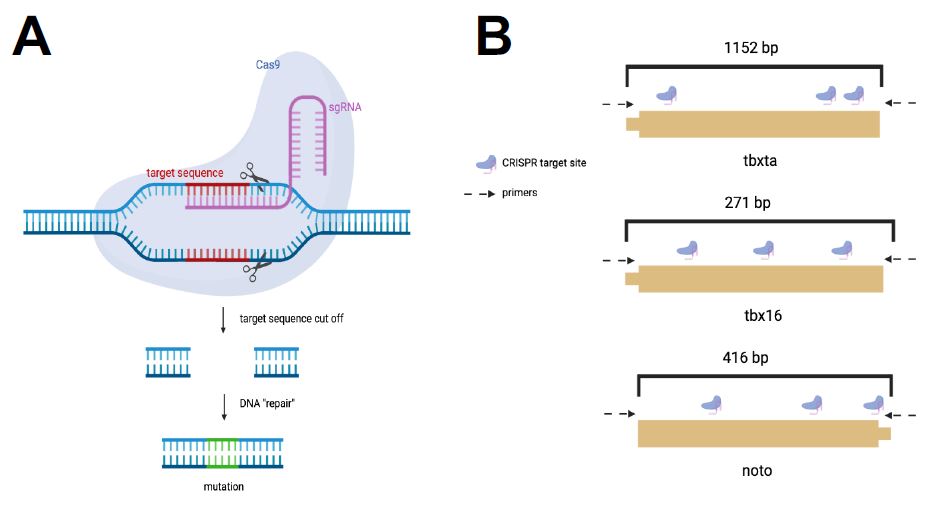
| Figure 2: CRISPR Cas-9 System for Mesoderm Perturbations. I used the CRISPR-Cas gene editing system to induce mutants in the three mesoderm transcription factors. A. The CRISPR system targets unique gRNA sequences to induce mutations at that genomic site. B. A gRNA sequence with three cut sites were designed for each transcription factor. |
A sequence of varying base-pair length was selected for tbxta, tbx16, and noto with three target sites per sequence based on their assigned mutability efficiency scores (Figure 2b). In total, three gRNAs were pooled together for each of the four genes and used to create the gene’s corresponding injection mixes. The injection mixes were individually created to perturb each gene of interest. Once the embryos were injected with the injection mix, mutant embryos were allowed to develop until 24 hours post fertilization (hpf) and were then observed for the expected phenotypes.
Figure 3a demonstrates the mutant phenotypes of the three gene perturbations, tbxta, tbx16, and noto. The tbxta mutants displays a shortened/lack of tail; tbx16 mutants display a spade tail, where muscle cells are over-differentiated in the tail; mutants of the noto condition display a lack of notochord and fused somites; and tyr mutants only have pigmentation loss as their observed phenotype. Through my experiments, I found that a consistent concentration used for the gRNAs across the conditions did not always yield healthy embryos with its expected mutant phenotype.
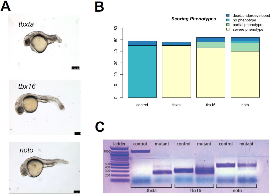
| Figure 3: Generation of CRISPR mutants. A. noto, tbxta, and tbx16 mutants with the expected mutant phenotype was generated through the CRISPR-Cas9 system. B. After calibration, my CRISPR injections yielded a high success rate of severe mutant phenotypes: noto injections showed a success rate of 90.38%, tbx16 with 92.31%, and tbxta with 93.75%. C. The mutants were confirmed to have mutations in the genomic level through the difference in band sizes between control and mutant embryos per condition corresponding to the CRISPR cut sites previously designed. |
Therefore, calibrations were performed in a series of injections with varying gRNA concentrations for each gene. The standard protocol for the injection mix called for 1.5 ul of gRNA, but that led to embryo death and toxicity for tbxta mutant embryos, while tbx16 and noto embryos did not display its appropriate mutant phenotype at 24hpf. After a series of calibration experiments, I determined that tbxta called for 1.0 ul gRNA with 0.5 ul purified H2O with only 2 puffs of injection mix during the injection, and tbx16 and noto required 1.5 ul gRNA with 3-4 puffs during injection. My final calibration for the injection mixes of the CRISPR-Cas9 protocol yielded a high success rate, as displayed in Figure 2c; only few of the injected embryos were dead and underdeveloped or were observed as wildtype, and a significant majority demonstrated a severe, expected phenotype. The success rates were quite high across all conditions: noto with 90.38%, tbx16 with 92.31%, and tbxta with 93.75%.
The CRISPR-Cas9 protocol I optimized yielded mutant embryos with the appropriate phenotypes, but I wanted to confirm that the mutations had occurred in the genes I targeted, using PCR and gel electrophoresis. Gel electrophoresis was used to visualize the mutations and differences present in the gene expression between wildtype embryos and mutant embryos. I performed a polymerase chain reaction to amplify the genomic DNA extracted from each condition’s mutant embryos before being visualized on the gel. I generated primers to correspond to each gRNA’s cut sites that were previously designed (Figure 1b). These primers were applied to wildtype and mutant embryos; the mutations that would have occurred in the mutants would have been in the genomic locations specified by the primers. In each perturbation condition, the gel visualized differences in DNA band sizes between the control and mutant, suggesting that mutations occurred in the genomic level (Figure 2e). These differences in band sizes corresponded to the gRNA cut sites: there is a large difference between the bp length of the tbxta mutant band versus the control band, which corresponds with the large distance between the first two target cut sites in the gRNA designed for tbxta. Similarly, the relatively equal spacing between the three cut sites in the noto and tbx16 gRNAs are consistent with the various and similar length of band sizes presented in the mutant columns.
- Single-Cell Analysis
10X Genomics scRNA-sequencing outputs raw genomic data for each of the perturbed conditions that first had to be aligned to a zebrafish transcriptome which aligns the RNA reads to the appropriate genomic location. I chose to align the raw single-cell data to the Lawson transcriptome, which was stated to better quantify 3’ and 5’ UTRs to represent the zebrafish genome more thoroughly (Lawson et al, 2020). The now aligned RNA reads were put through Seurat’s single-cell analysis workflow (Figure 4a).
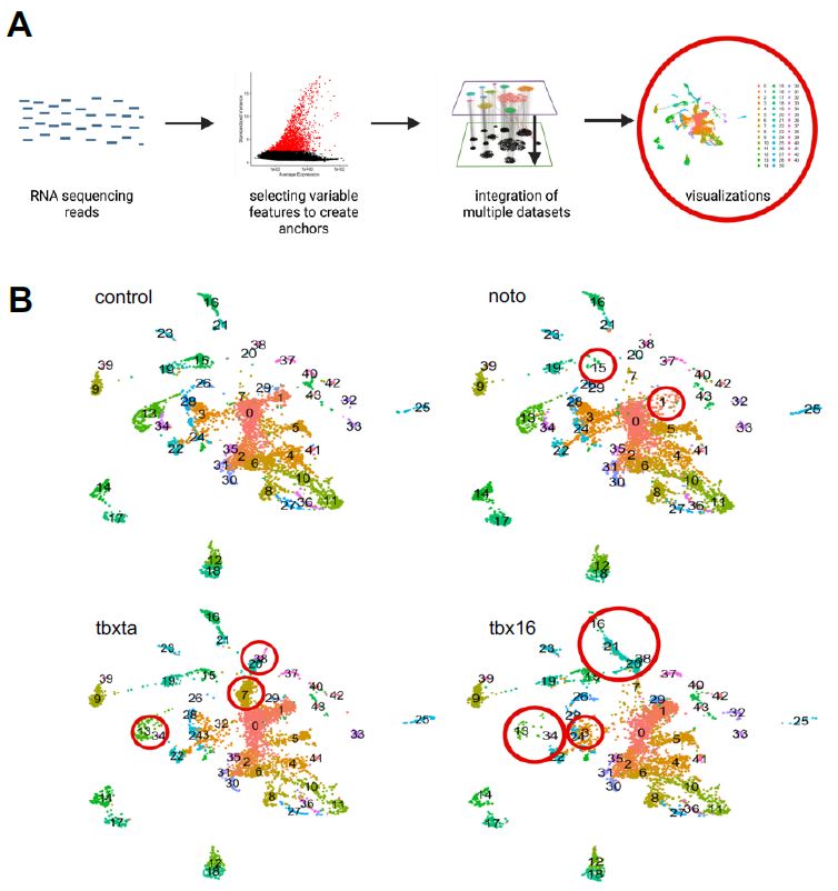
Figure 4: A single-cell CRISPR gene perturbation analysis workflow. The RNA sequencing reads are put through the Satija Lab’s Seurat workflow for clustering and integration (described in methods). Ultimately visualizations can be generated to understand the cell populations and how it differs between perturbed conditions.
Through a series of quality control, filtering, and normalization methods, single cells in each sample were clustered together based on similar gene expression to create sub-populations or “clusters”. A data integration across all four samples was also implemented to identify cell types present in all conditions, enabling the detection of similarities and differences between samples; essentially, I developed clusters that aggregate cells with similar gene expression across all the sample conditions (control, tbxta, tbx16, and noto). UMAP visualizations were generated for the integrated object, split up by sample condition, as shown in Figure 4b. Visually, I was able to see differences in density of clusters in mutant conditions compared to the control, as demonstrated by the red circles in panel 4b.
However, the arbitrary numbered identification given by Seurat does not attribute any information regarding cell types to each cluster, so these visual differences and similarities in cell abundance did not initially yield useful information. Reference cell atlases exist that identify the top marker genes that establish a cell type, which could be manually applied to sample data, but it is inefficient and not precise. Therefore, I developed a label transfer method that transfers cell type labels of an existing reference cell atlas to my unlabeled integrated single-cell data (Figure 5). I developed this framework around the two inputs I was having difficulty putting together: the FindAllMarkers output that lists the highly differentiated markers for each cluster of the integrated object and the reference cell atlas that contains the top 20 markers that establish a cell type. I used the Wagner annotation for 24hpf zebrafish embryos (Wagner et al., 2018). This annotation was recently developed by the Wagner Lab to profile the top 20 genetic markers that establish cell types of zebrafish at the 24hpf time point; because of this time point, I decided to use this annotation as my reference cell atlas. I created a loop that essentially compares each list of markers for a cell type against each list of markers for an unlabeled cluster. The loop determines a match vector that is the number of matches between each cell type and each cluster, theorizing that a high match vector equates a most likely cell type identification. To visualize these match vectors, a heatmap, as displayed in Figure 5, was generated to display the magnitude of matches between the two data frames. Finally, these clusters can then be renamed in the object and applied to the UMAP plot, so the cell abundance differences have a cell type attribution.
|
|
| Figure 5: Label Transfer Schematic. An agnostic computational framework that transfers cell type labels from a reference atlas onto a perturbed sample’s dataset. The final output is a heatmap visualizing the magnitude of correlation between the query sample’s highly differentiated markers for each cluster and the reference atlas’s markers for a defined cell type. |
Stated previously, the label transfer method uses the highly differentiated markers for each cluster generated from the integrated dataset workflow. In this Seurat workflow, the dimensionality chosen when the FindClusters function is used forces Seurat to create a certain amount of clusters for a dataset. For example, using resolution = 1.5, which is Seurat’s standard, yields a greater number of clusters while resolution = 1.0 forces a lower number of clusters; this resolution refines what is considered enough for cells to have similar gene expression and be in a same sub-population. To test the robustness of my label transfer framework when the cluster input varies, I tested three different scenarios in which the number of clusters, and therefore what cells constitute each cluster, are different (Figure 6a).
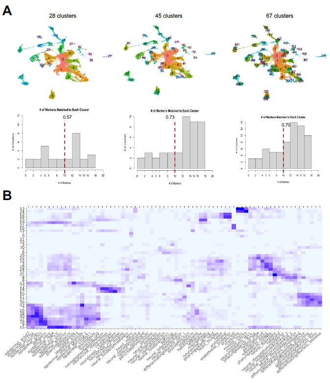
| Figure 6: Cluster/Marker Distribution. A. I tested different dimensionalities of clusters and its corresponding markers to see how identification of cell types vary. A mean amount of clusters doesn’t force the cells to under/over cluster, meaning the cells that don’t share as much gene expression do not congregate together. B. Using the 45 clusters, I generated each cluster’s cell type identification, as shown in the heatmap output of the label transfer framework. The x-axis is the cell type labels from the reference atlas and the y-axis is the unlabeled clusters. A darker hue of square indicates a larger, or better, match magnitude, with the maximum being 20 and minimum of 0. |
The first scenario is where I used resolution = 0.5 to force a lower number of clusters compared to the standard at 28 clusters. The second scenario used the standard of resolution = 1.5 to obtain 45 clusters, and the third scenario used resolution = 3.2 to yield 67 clusters. After obtaining the FindAllMarkers data set for each of these scenarios, I individually inputted them to my label transfer method with the Wagner reference to see how the identifications of cell types are altered. I quantified having a better identification by determining how many clusters demonstrated a match vector of at least 10, as a match vector of 20 would be considered a perfect match based on the construction of the Wagner reference. Generally, forcing the integrated object to have a cluster dimensionality closer to Seurat’s standard allowed for better identification of clusters with cell types. From this determination, I chose to use the resolution = 1.5, with 45 clusters, for further single-cell analysis. I finally was able to determine the cell type labels of the sub-populations of my sample dataset, as shown in the heatmap of Figure 6b.
- Quantifying Cell Abundance Differences
With the cell type identities of my sample dataset determined, I wanted to quantify the visual differences I had previously seen in cell type abundances for each genotype. To do this, I used a log10 transformation calculation, comparing each mutant condition to the control condition to see if there were increases, decreases, or no changes in cell abundance in the mutants. Figure 7 displays this information as a heatmap.
|
||
| Figure 7: Quantifying Differences in Cell Abundance. A log10 difference was used to compare each mutant condition to the control. The scale is -1 to 1, with -1 being a decrease in mutant’s cell type compared to control and +1 being an increase in mutant compared to control. |
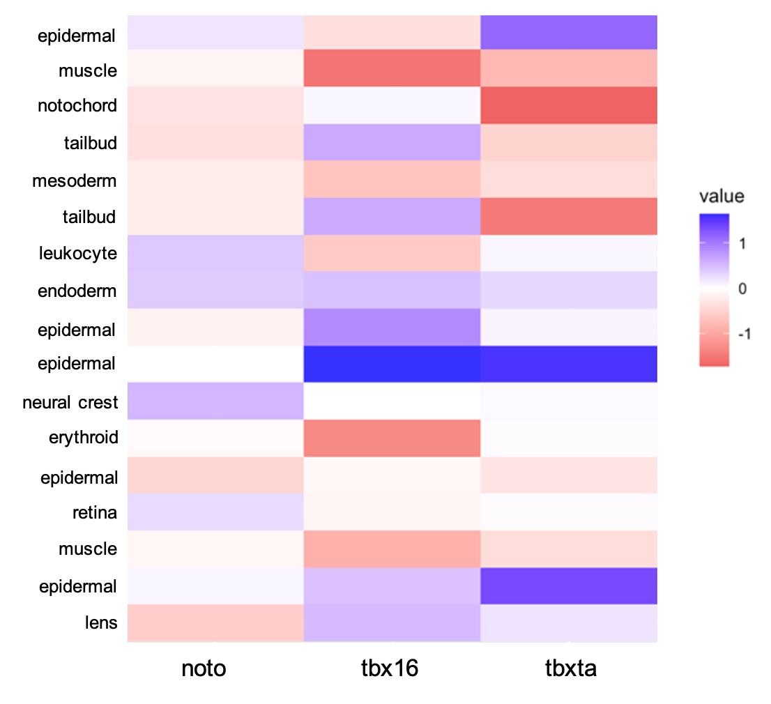
There are differences in cell abundance that were expected by the nature of the perturbation and what we know of these transcription factors previously: tbx16 had a large decrease in muscle cells which corresponds to cells creating the knot-like formation in the tail, rather than differentiating as muscle, also correlating with the increase in tailbud cells. tbxta presented a decrease in notochord and tailbud cells that matches with its loss of tail phenotype. tbx16 has also been speculated to have interactions in the development of the heart, making the loss of erythroid cells an interesting observation (Griffin & Kimelman, 2002). Compared to the other two mutant conditions, noto overall displayed a less severe amount of cell abundance differences when compared against the control. Throughout the mutant conditions, all mesoderm cells decreased in comparison to the control, which is expected in these overall mesoderm-perturbed conditions. There is a shared increase in epidermal cells in all the mutant conditions, which reflects a potential phenomenon, perhaps cells are forced to develop other cell types such as epidermis when they cannot form mesendoderm. This observation could support the reasoning behind cells developing to ectoderm versus mesendoderm.
An interesting observation that has not been previously seen is the shared increase in endodermal cells. Compared to all other cell types that show an increase or decrease in cell abundance, endoderm has the greatest logarithmic increase in all three mutant conditions. noto was determined to have a 0.39-fold increase in cell abundance, tbxta with 0.30, and tbx16 with 0.46. Because the increase in cell abundance seemed significant relative to differences seen in other cell types, I chose to further investigate this observation. I have preliminarily hypothesized that cells might default to endoderm when the decision to develop mesoderm is being denied. It was difficult to determine the actual significance of this observation, therefore I decided to use different experimental methods to test my hypotheses. Right now, I am performing an in-situ hybridization with the sox17 RNA probe, a classic marker for endoderm. I believe this validation will be further evidence to either support or not support my hypothesis.
DISCUSSION
The broad objective of my project was to understand how the mesodermal gene regulatory network, consisting of tbxta, tbx16, and noto, functions to specify different layers of the mesoderm during early development. As stated previously, these three transcription factors are classic markers for the mesodermal layer, having been studied to see how they each contribute to developing key mesodermal derivatives such as the notochord and somites. I wanted to apply the novel technologies of CRISPR gene editing and single-cell sequencing to answering this question, and essentially shine a new perspective on answering a classic question. I developed and optimized several protocols, experimental and computational, for the combining of CRISPR mutagenesis with scRNA-seq techniques in this pursuit to study the mesoderm. The model I have developed streamlines the generation of mesodermal mutants using CRISPR and the analysis of the molecular profiles of individual cells within each mutant. Developing this model first began with trying to recapitulate what is known about these transcription factors, establishing the efficacy of this combination of methods. The mutants that were generated using the CRISPR system was done with the goal to reflect each TFs already established mutant phenotype in previous literature, where older genetic tools were used such as morpholinos to create those mutants. Similarly, I was expecting the mutant phenotypes to be reflected in the single-cell data, in which the cell types that were visually perturbed were also affected in the single-cell level.
Like CRISPR gene editing, single-cell sequencing analysis required a lot of troubleshooting through experiencing the limitations of the novelty of the technology. I experienced this greatly in trying to identify the sub-populations of my samples, so I could efficiently understand how different cell types are influenced after undergoing a perturbation. I initially tried to label the sub-populations of my samples by hand, comparing the top 20 expressed markers within each cluster to the top 20 markers that establish a cell type; this method was quite tedious and allowed for error. This difficulty in doing so led me to develop a computational method that transfers labels in an automatic and unsupervised fashion. The label transfer method was also written in a matter where it is compatible with any reference cell atlas and any FindAllMarkers output, so it is transferable to others who would like to quickly identify the sub-populations in their single-cell dataset regardless of what timepoint or type of embryos they are working with. I adapted the framework to be a function in R and is downloadable through the Gagnon Lab’s GitHub, which is linked in the appendix.
The cell abundance differences I observed from my single-cell data demonstrated known changes in cell types, like the decrease in notochord for tbxta and decrease of erythroid cells in tbx16. I also observed changes in cell types that haven’t been established in previous literature, such as the general increase in endodermal cells across all the mesoderm-perturbed conditions. However, it was difficult to determine the significance of these changes I observed, as my experiment did not allow for replicates of single-cell data. This meant that calculating significance using statistical methods was not a fruitful avenue to go down; instead, I chose a few hypotheses, one being the endodermal hypothesis, and am finding different ways to test them. The experimental pathway I have chosen to confirm these hypotheses is to visualize endodermal gene expression through in-situ hybridization (Thisse & Thisse, 2008). The in-situ hybridization method allows me to visualize the RNA of a gene of choice in the mutant embryos I have generated. I am using a sox17, a classic endodermal marker, probe to visualize its gene expression in the mutant and control embryos to see if there is an increase in endodermal expression.
I hope to use the optimized methods I have developed using CRISPR and scRNA-seq technologies to further understand the mesodermal gene regulatory network. The beginning of this project was founded in exploring the different interactions tbxta, noto, and tbx16 have with each other, specifically how they worked synergistically and antagonistically to overall develop the mesodermal layer. I would also like to identify redundancies in this network by inducing double and triple mutants using this optimized pipeline. I believe introducing double and triple mutants will allow for me to observe the presence of synergistic and antagonistic interactions between the pairs of transcription factor perturbations. Beyond tbxta, noto, and tbx16, there are other pathways and genes that influence mesoderm specification, it would be interesting to apply the methods I have developed to different genes and transcription factors to understand early development of the zebrafish.
ACKNOWLEDGEMENTS
Thank you so much to Dr. James Gagnon for guiding me through the project and introducing me to the world of genetics and developmental biology research. Thank you for encouraging and supporting me academically and personally throughout my undergraduate career. I would also like to thank Sheng Wang and Clay Carey for providing me with your support in teaching me how to run lab protocols and troubleshoot my computational work. I could not have done it without all of you.
REFERENCES
- Campbell, A., Anderson, W. W., & Jones, E. W. (2005). Molecular Genetics of Axis Formation Zebrafish. In Annual Review of Genetics (pp. 579–581). Essay, Annual Reviews.
- Griffin, K. J., & Kimelman, D. (2002). One-Eyed Pinhead and Spadetail are essential for heart and somite formation. Nature cell biology, 4(10), 821–825. https://doi.org/10.1038/ncb862
- Hoffman, P., & Satija Lab. (2023, March 27). Seurat – Guided Clustering Tutorial. • Seurat. Retrieved from https://satijalab.org/seurat/articles/pbmc3k_tutorial.html
- Jones, C. M., Kuehn, M. R., Hogan, B. L., Smith, J. C., & Wright, C. V. (1995). Nodal-related signals induce axial mesoderm and dorsalize mesoderm during gastrulation. Development, 121(11), 3651–3662. https://doi.org/10.1242/dev.121.11.3651
- Lawson, N. D., Li, R., Shin, M., Grosse, A., Yukselen, O., Stone, O. A., Kucukural, A., & Zhu, L. (2020). An improved zebrafish transcriptome annotation for sensitive and comprehensive detection of cell type-specific genes. eLife, 9, e55792. https://doi.org/10.7554/eLife.55792
- Payumo, A. Y., McQuade, L. E., Walker, W. J., Yamazoe, S., & Chen, J. K. (2016). Tbx16 regulates hox gene activation in mesodermal progenitor cells. Nature chemical biology, 12(9), 694–701. https://doi.org/10.1038/nchembio.2124
- Ran, F. A., Hsu, P. D., Wright, J., Agarwala, V., Scott, D. A., & Zhang, F. (2013). Genome engineering using the CRISPR-Cas9 system. Nature protocols, 8(11), 2281–2308. https://doi.org/10.1038/nprot.2013.143
- Schulte-Merker, S., van Eeden, F. J., Halpern, M. E., Kimmel, C. B., & Nüsslein-Volhard, C. (1994). no tail (ntl) is the zebrafish homologue of the mouse T (Brachyury) gene. Development (Cambridge, England), 120(4), 1009–1015. https://doi.org/10.1242/dev.120.4.1009
- Stemple, D. L., Solnica-Krezel, L., Zwartkruis, F., Neuhauss, S. C., Schier, A. F., Malicki, J., Stainier, D. Y., Abdelilah, S., Rangini, Z., Mountcastle-Shah, E., & Driever, W. (1996). Mutations affecting development of the notochord in zebrafish. Development (Cambridge, England), 123, 117–128. https://doi.org/10.1242/dev.123.1.117
- Thisse, C., & Thisse, B. (2008). High-resolution in situ hybridization to whole-mount zebrafish embryos. Nature protocols, 3(1), 59–69. https://doi.org/10.1038/nprot.2007.514
- Wagner, D. E., Weinreb, C., Collins, Z. M., Briggs, J. A., Megason, S. G., & Klein, A. M. (2018). Single-cell mapping of gene expression landscapes and lineage in the zebrafish embryo. Science (New York, N.Y.), 360(6392), 981–987. https://doi.org/10.1126/science.aar4362
