College of Science
54 The Emergence of Chaos in Lasers
Steven Marz (University of Utah)
Faculty Mentor: Elena Cherkaev (Mathematics, University of Utah)
1 Introduction
Since their creation in the 1960s, lasers have become valuable tools not only in the scientific com- munity but in daily life (laser pointers, barcode scanners, printers, communication systems, etc.). Most lasers are operated in what is known as the lasing regime, where the emitted light is co- herent, meaning it has well defined phase, amplitude, and wavelength. Additionally, lasers can operate chaotically. This chaotic regime is less commonly used but is actively researched and has applications in random number generation, communications, and metrology [5].
Chaos is well known to only appear in systems that are described by a system of differential equations with a minimum of three dimensions. In some regimes, the behavior of a laser can be modelled with a two (or even one) dimensional system of equations [1]. More complicated and precise models increase the number of dimensions of the system of equations and thus can describe chaotic laser operation [1] [2]. This paper will compare a two dimensional model of a laser to a three dimensional model and explore the emergence of chaos in the three dimensional model.
2 Models
The two models presented here both describe lasers but focus on different characteristics of the laser. Additionally, we will be focusing on three regimes lasers can operate in: non-lasing, lasing, and chaotic. Neither of these models capture the full complexity of laser operation, and examples of more intricate laser operation abound [3] [4] [5]. However, these simulations do serve to demonstrate the emergence of chaotic behavior even in greatly simplified models of lasers.
2.1 Two-Dimensional
The two-dimensional system of equations is presented in [1]. It is a coupled two-dimensional system of ordinary differential equations, given by eqs. (1) and (2).
n ̇ = GnN − kn (1)
N ̇ =−GnN−fN+p (2)
In this model, n represents photon number, N represents the number of excited atoms, n ̇ and N ̇ represent the time derivatives of n and N, G is the gain of the laser, k is the loss rate of photons, f is the decay rate of the excited state, and p is the strength of the pump. Since the focus of this paper is analyzing the behavior of the solutions of these equations, we will rewrite (1) and (2) in a simpler dimensionless form via the substitutions x=Gn/k, y=GN/k, a=f/k, τ=kt, and b=Gp/k2 [1].
Now, (1) and (2) are rewritten as (3) and (4).
dx / dτ = x(y – 1) (3)
dy/dτ = -y(x + a) + b (4)
As mentioned earlier, chaos does not appear in this model since it is two-dimensional. However, it can describe the non-lasing and lasing regimes. Here, the transition from non-lasing to lasing occurs when b becomes larger than a. Once this occurs, x, the dimensionless equivalent to photon number, will approach b−a as time goes to infinity. The transition from non-lasing to lasing is shown in fig. 1, where (3) and (4) were numerically integrated using a fifth order Runge-Kutta method in Python to generate the plots. In all situations, x and y were initially set to 1. Fig. 1(a) shows results from a simulation which used a = 1.5, b = 1.0, 1(b) shows results with a = 1.0, b = 1.0, and 1(c) shows results with a = 1.0, b = 1.5.
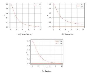
Fig. 1 clearly shows x going to zero below the transition, slowly going to zero at the transition point, and approaching the expected finite value above the transition point.
2.2 Maxwell-Bloch Equations
The three-dimensional equations studied here are known as the Maxwell-Bloch equations. Eqs. (5)- (7) show the dimensionless form, as presented in [1] and [2]. These equations were also numerically integrated using fifth order Runge-Kutta method in Python to generate the plots shown later in this section.
E ̇ = κ(P − E) (5)
P ̇ =γ1(ED−P) (6)
D ̇ =γ2(λ+1−D−λEP) (7)
This model treats the laser semi-classically and thus models the electric field, E, instead of the photon number, n. The other two quantities, P and D, represent the mean polarization of the atoms and the population inversion, respectively. Electric field and polarization are, in general, vector valued. Here we assume that they always point in one direction and thus E and P represent the magnitude of these vectors in that direction. κ corresponds to the decay rate from light transmission, γ1 corresponds to the rate of depolarization, γ2 is the population inversion decay rate, and λ is related to the pump strength. Here, λ < 0 corresponds to a pump which is not strong enough to sustain population inversion, the collective excitation of the lasing medium.
The non-lasing regime, where E tends towards zero, is thus defined by setting λ < 0. This roughly corresponds to the situation where the strength of the pump is too low to force lasing behavior and either incoherent emission, like a lamp, or no light emission at all, is the result. Fig. 2 shows electric field E in this regime, where initially E = P = D = 0.5, κ = γ1 = γ2 = 1, and λ = −1. Fig. 2(b) shows that the trajectory quickly approaches the origin, hence no coherent electric field is produced and lasing does not occur.
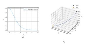
Figure 2
The lasing regime is defined by 0 ≤ λ < λH, where λH = κ ![]() −1 so long as κ>γ2 + γ1 In this regime, E will exhibit damped oscillations around 1 or -1. This stable equilibrium corresponds to a coherent, polarized electric field and hence proper lasing. Fig. 3 shows a situation whereEoscillatesaround1,withE=P=D=0.5initiallyandκ=γ1 =γ2 =λ=1. Additionally, the time length was extended to better capture the behavior.
−1 so long as κ>γ2 + γ1 In this regime, E will exhibit damped oscillations around 1 or -1. This stable equilibrium corresponds to a coherent, polarized electric field and hence proper lasing. Fig. 3 shows a situation whereEoscillatesaround1,withE=P=D=0.5initiallyandκ=γ1 =γ2 =λ=1. Additionally, the time length was extended to better capture the behavior.
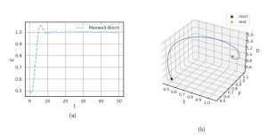
Figure 3
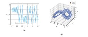
The Maxwell-Bloch equations are capable of demonstrating a third chaotic regime which the two-dimensional equations were unable to predict. This regime is defined by λ > λH and κ > γ2+γ1. Once this condition is fulfilled, the system undergoes a subcritical Hopf bifurcation. As shown in fig. 4, this regime has E aperiodically switching between oscillations around 1 and -1. This figure uses E=P =D=0.5 initially along with γ1 =γ2 =1, κ=3, and λ=21.
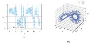
Figure 4
In order to demonstrate the sensitive dependence on initial conditions, fig. 5 shows the results of a simulation which used the same parameters as fig. 4, but with E now set to 0.51.
A comparison of figs. 4 and 5 clearly demonstrates sensitive dependence on initial conditions, as expected in a chaotic system. The final points are at different positions in phase space and the timing of flips between 1 and -1 become completely uncorrelated.
What this theory physically predicts is an operating regime in which a laser emits monochromatic light which chaotically fluctuates in intensity and switches polarization. In actuality, this is quite hard to realize experimentally. Most demonstrations of chaos in lasers arise in more complicated situations which this model does not accurately describe [5]. As shown in [3], more complicated laser systems show more than three operating regimes and show different types of chaotic behavior. Chaotic behavior similar to that predicted by the model described here is demonstrated experimentally in [4], which was published decades after the theoretical prediction of this sort of chaos.
The strange attractor that shows up in the chaotic regime is remarkably similar to the famous Lorenz butterfly, a strange attractor which arises from the Lorenz system given in eqs. (8)-(10). In
fact, as shown in [1] and [2], the transformation t → (σ/κ) t′, E → αx, P → αy, D → (r − z), γ1 → k/σ , γ2 → (κβ)/σ , and λ → r − 1, where ![]() , exactly transforms the Maxwell-Bloch equation into the Lorenz system.
, exactly transforms the Maxwell-Bloch equation into the Lorenz system.
x ̇ = σ(y − x) (8)
y ̇ = rx − y − xz (9)
z ̇ = xy − bz (10)
3 Conclusion
The modelling of lasers leads to sets of equations which work as wonderful examples of the emergence of chaos. Both models here were able to describe the primary lasing and non-lasing regimes of laser operation, but the simpler model left out key details which allow for the exploration of a chaotic laser. This serves as an example of the way new behaviors can be revealed through more detailed modelling and simulation.
References
- Strogatz, S.H., Nonlinear Dynamics and Chaos: With Applications to Physics, Biology, Chemisty, and Engineering, 2nd edition, 2015.
- Haken, H., Analogy between higher instabilities in fluids and lasers, Physics Letters, Vol. 53A, No. 1, 1975.
- Frese et al., Routes to chaos in a class-B laser coupled to a neutral resonator, 25 April, 2022.
- Virte et al., Deterministic polarization chaos from a laser diode, Nature Photonics, November, 2012.
- M. Sciamanna, K. A. Shore, Physics and applications of laser diode chaos, Nature Photonics, February, 2015
