College of Engineering
17 Investigating Curvature Induced Circumferential Drifts to Improve the 3D Reconstruction of a Deployed Stent
Michael Keyser (University of Utah) and Lucas Timmins (Biomedical Engineering, University of Utah)
Faculty Mentor: Lucas Timmins (Biomedical Engineering, University of Utah)
Introduction
Coronary Heart Disease (CHD) is one of the most common causes of death in the United States. It accounts for 370,000 deaths annually. Various lifestyle choices, such as maintaining a healthy diet, exercising, not smoking, and limiting alcohol consumption to moderate amounts reduce the risk of CHD, but sometimes proper lifestyle choices are not sufficient [1]. CHD is caused by a buildup of plaque in the arteries called atherosclerosis. The plaque blocks blood flow to the myocardial tissue, which can lead to a heart attack. Clinicians use stents to open arteries blocked by plaque to restore blood flow in the affected artery. Stenting arteries is generally successful, but there is up to a 30% chance the stent will fail due to the ingrowth of tissue that re- blocks the vessel – termed restenosis [2].
Biomechanics has been shown to play a key role in stent failure [3]. Currently, studies that investigate the biomechanics in stented regions are limited to general cases because they lack the ability to model the in vivo geometry of the stented region. Elliott et al. developed a technique that utilizes optical coherence tomography (OCT) imaging data to reconstruct the in vivo deployed stent and vessel geometry [4].
In summary, the stent struts are reliably identified in OCT images [5]. Through fusion with biplane angiography [6], the stent struts are matched to the shape of the vessel to create a sparse representation of the known locations of the stent after being deployed, herein OCT point cloud. The physical dimensions of the stent are known, so an accurate model of the stent can be constructed and fitted to the OCT point cloud, through a constrained deformation process called diffeomorphic mapping [4]. Once the diffeomorphic mapping is complete, an accurate geometry of the patient specific stent has been reconstructed and the biomechanics in the region can be studied. The accuracy of the OCT point cloud is integral to the process because the diffeomorphic mapping assumes the OCT point cloud is correct.
A rotational shift was observed in the collected OCT images. The curvature of the vessel caused the drift in OCT images. This imaging artifact is referred to as circumferential drift. OCT images can be adjusted prior to strut identification to correct for the effects of circumferential drift. An experimental testbed with three channels of constant curvature were scanned and the circumferential drift was measured across the OCT stack. The circumferential drift was observed in the direction of the curve. The normal vector of a curve in the Frenet-Serret frame (TNB) points inwards on a curve. Finally, the Frenet-Serret frame (TNB frame) was calculated at each point along the centerline to determine the direction of circumferential drift.
Methods
A. Algorithm for Identifying OCT Image Angle
Three separate channels were drilled out of a Deldrin® experimental test bed using a CNC- machine. The three separate channels had curvatures of = 20-1mm, 30-1mm, and 60-1mm, respectively. The channels were drilled to appear as a ‘U’ when viewing the OCT images in Cartesian. An OCT catheter (DragonflyTM OPTISTM, Abbott Vascular) was inserted into each channel to acquire OCT images. The channels were scanned in both “high-resolution” and “survey” mode where the distance between OCT frames is 0.1 mm and 0.2 mm, respectively.
The top of the ‘U’ was identified and its angular change across images was tracked. Figure 1 shows there is a faint linear section along the top of the ‘U’. The angle of the faint section is the angle of the OCT frame.
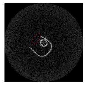
Figure 1. OCT image of experimental testbed in Cartesian.
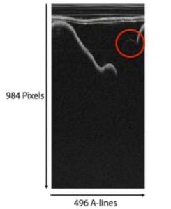
Figure 2. OCT image of experimental testbed in polar.
The points making up the faint line were identified by analyzing the OCT image in its polar and Cartesian views. First, the OCT image was viewed as a polar image. Each OCT image has 496 axial lines (A-lines) and a depth of 984 pixels per image as shown in figure 2. The peak- intensity depth was identified in each A-line and was filtered with intensities greater than 25% of the mean intensity were removed. Noise was removed by filtering out depths where intensities changed by more than 5 between adjacent depths. Intensities were then filtered to consider depths within 20 below the median intensity and one standard deviation above the mean intensity. The remaining depths consisted of the faint linear section along the top of the ‘U’.
The OCT image was converted to Cartesian where the faint section appears linear. A line was fit through the points. Outliers were removed and a new line of best fit was calculated up to three times. The leftmost and rightmost of the remaining points were chosen to calculate the angle of a line passing through the points. Figure 3 shows the line used to compute the angle of the OCT image.
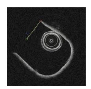
Figure 3. OCT image with the selected line shown in yellow.
B. Calculating Circumferential Drift
The angles of the OCT images were plotted against the position in the OCT stack as shown in figure 4.
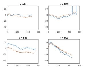
Figure 4. Image angle plotted across the OCT stack.
Angles were filtered using a Gaussian filter. Noise created by random rotation was present in many of the measurements due to the imaging probe rubbing against the channel, which is common in OCT scans. A region without substantial noise was selected and its corresponding set of OCT images were inspected to confirm a smooth rotation. The smooth region had an approximately linear slope. A line was fit through the region and the slope of the line was the circumferential drift per frame. The drift per frame was multiplied by the number of frames in a millimeter (10 frames/mm for “high-resolution”, 5 frames/mm for “survey” mode) to get the circumferential drift per mm. The average of the circumferential drift per mm in the “high-resolution” and “survey” modes was reported as the circumferential drift per mm.
Tracking the angular change of the ‘U’ quantified the magnitude of the circumferential drift but did not account for the direction of the circumferential drift. OCT images were manually reviewed, and the circumferential drift was observed towards the inside of the curve. Each OCT scan is accompanied by a biplane angiogram that provides 3D centerline data for the OCT stack OCT images were arranged in 3D space along the centerline as shown in figure 5. The TNB framework was calculated for each OCT frame along the centerline. The normal vector points inwards on the curve (i.e., in the direction of circumferential drift) and calculating the angle between the normal vector and the vertical of the OCT image quantifies the direction of the circumferential drift. If the normal vector is to the left of the vertical, the circumferential drift is counterclockwise. The normal vector right of the vertical indicated the circumferential drift was clockwise.
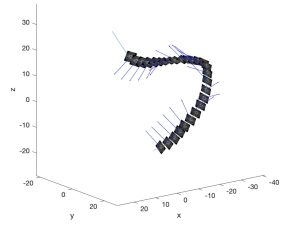
Figure 5. OCT images properly aligned in 3D space using the centerline from an angiogram.
C. Correcting the Full Stent Reconstruction to Account for Circumferential Drifts
A circumferential drift correction was implemented into the method developed by Elliot et al. [4]. First, the circumferential drift of each OCT image was calculated independent of the stent reconstruction process. The cumulative circumferential drift was calculated for each image by summing the drifts of all preceding images in the stack. Drifts could be negative due to their direction and summing preceding drifts accounts for changes in drift direction. Images were adjusted for drift by circularly shifting the A-lines in the polar image (circular shift means A- lines “wrap-around” when shifted, e.g. A-line 496 will move to A-line 1 when shifting down 1). Shifting the A-lines in a polar OCT image are equivalent to rotating the OCT image where one A-line is equivalent to 0.726°. Shifting A-lines was chosen over rotation in Cartesian to avoid changing pixel values from interpolation present in image rotation algorithms. Pixel values must not be altered to not affect the performance of the stent strut identification algorithm. Once all images in the OCT stack were adjusted, stent strut identification could begin.
Results
A. Formula Relating Curvature to Circumferential Drift
The circumferential drift was found to be -0.1719°/mm, -0.5979°/mm, -0.9727°/mm, and – 1.1243°/mm for curvatures of 0, 1/20, 1/30, and 1/60 mm-1, respectively. The straight channel (curvature of 0 mm-1) had a drift of -0.1719°/mm because of catheter movement, which is an acceptable noise level. Figure 6 shows the drifts were plotted against curvature and the line of best fit gave the formula relating curvature to circumferential drift in degrees per millimeter where κ is curvature and is the circumferential drift. Equation 1 is the line of best fit and the formula relating curvature to circumferential drift.
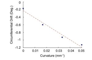
Figure 6. Plot showing the linear relationship between curvature and circumferential drift.
𝜃 = −19.12𝜅 − 0.227
Equation 1. Relationship between curvature and circumferential drift.
B. Validating Angle Correctness Algorithm
The angle identification algorithm performance was compared to a ‘gold standard’ set by manual inspection. 50 OCT images were randomly chosen from two OCT scans (50 from each scan) and were manually inspected. The angle of each image was manually calculated using the Angle Tool in ImageJ. A Bland-Altman plot and Lin’s concordance correlation coefficient (CCC) showed a strong agreement between the algorithm and the ‘gold standard.’ Figure 7 shows there is no systematic difference between the algorithm and ‘gold standard.’ The CCC was 0.99103, showing there is strong agreement between the algorithm and ‘gold standard.’
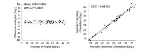
Figure 7. Bland-Altman and CCC plots validating the results of the angle detecting algorithm.
Conclusion
Existing stent reconstructions suffer from curvature induced circumferential drifts. We successfully developed a framework that quantified the magnitude and direction of the circumferential drift and adjusted OCT images to counteract the effects of the circumferential drift. The circumferential drift was found to be -0.1719°/mm, -0.5979°/mm, -0.9727°/mm, and – 1.1243°/mm for curvatures of 0, 1/20, 1/30, and 1/60 mm-1, respectively. Linear regression was used to relate curvature to circumferential drift given by equation 1. Future work will investigate the effects of circumferential drift corrections on the completed 3D stent reconstruction.
References
[1] Benjamin, E. J., Circ., vol 137, pp e67-e492, 2018.
[2] Cassese, S., Heart, vol. 100, no. 2, pp. 153–159, 2014.
[3] LaDisa Jr., J. F., Am. J. Physiol. Heart Circ. Physiol., vol. 288, no. 5, pp. H2465–H2475, 2005.
[4] Elliott, M. R., IEEE Trans. Med. Imaging, vol. 38, no. 3, pp. 710–720, 2019. [5] Chiastra, C., J. Cardiovasc. Transl. Res., pp. 1–17, 2017.
