26 Bohr’s Theory

Emission Spectrum of the Hydrogen Atom

The emission spectrum of atomic hydrogen is divided into a number of spectral series.

The emission spectrum of a chemical element or chemical compound is the spectrum of frequencies of electromagnetic radiation emitted by an atom’s electrons when they are returned to a lower energy state. Each element’s emission spectrum is unique, and therefore spectroscopy can be used to identify elements present in matter of unknown composition. Similarly, the emission spectra of molecules can be used in chemical analysis of substances.

The emission spectrum of atomic hydrogen is divided into a number of spectral series, with wavelengths given by the Rydberg formula: [latex]\frac{1}{\lambda_{vac}} = RZ^2 (\frac{1}{{n_1}^2} - \frac{1}{{n_2}^2})[/latex]

where R is the Rydberg constant (approximately 1.09737 x 10⁷ m^-1), [latex]\lambda _{vac}[/latex] is the wavelength of the light emitted in vacuum, Z is the atomic number, and n₁ and n₂ are integers representing the energy levels involved such that n₁ < n₂. All observed spectral lines are due to electrons moving between energy levels in the atom. The spectral series are important in astronomy for detecting the presence of hydrogen and calculating red shifts. Further series for hydrogen as well as other elements were discovered as spectroscopy techniques developed.

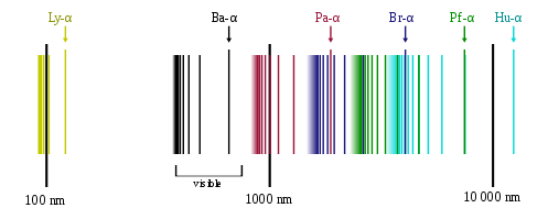
The line spectrum of hydrogen: Explain how the lines in the emission spectrum of hydrogen are related to electron energy levels.

The spectral lines are grouped into series according to n′. Lines are named sequentially starting from the longest wavelength/lowest frequency of the series using Greek letters within each series. For example, the 2 → 1 line is called Lyman-alpha (Ly-α), while the 7 → 3 line is called Paschen-delta (Pa-δ). Some hydrogen spectral lines fall outside these series, such as the 21 cm line (these correspond to much rarer atomic events such as hyperfine transitions). The fine structure also results in single spectral lines appearing as two or more closely grouped thinner lines due to relativistic corrections. Typically, one can only observe these series from pure hydrogen samples in a lab. Many of the lines are very faint and additional lines can be caused by other elements (such as helium if using sunlight or nitrogen in the air). Lines outside of the visible spectrum typically cannot be seen in observations of sunlight, as the atmosphere absorbs most infrared and ultraviolet wavelengths through the action of water vapor and ozone molecules respectively.

The Bohr Model

The Bohr model depicts atoms as small, positively charged nuclei surrounded by electrons in circular orbits.

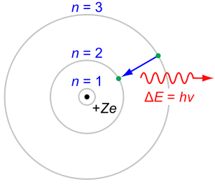
In atomic physics, the Bohr model depicts an atom as a small, positively charged nucleus surrounded by electrons. These electrons travel in circular orbits around the nucleus—similar in structure to the solar system, except electrostatic forces rather than gravity provide attraction.

The Rutherford–Bohr model of the hydrogen atom. In this view, electron orbits around the nucleus resemble that of planets around the sun in the solar system.

Development of the Bohr Model

The Bohr model was an improvement on the earlier cubic model (1902), the plum-pudding model (1904), the Saturnian model (1904), and the Rutherford model (1911). Since the Bohr model is a quantum -physics-based modification of the Rutherford model, many sources combine the two: the Rutherford–Bohr model.

Although it challenged the knowledge of classical physics, the model’s success lay in explaining the Rydberg formula for the spectral emission lines of atomic hydrogen. While the Rydberg formula had been known experimentally, it did not gain a theoretical underpinning until the Bohr model was introduced. Not only did the Bohr model explain the reason for the structure of the Rydberg formula, it also provided a justification for its empirical results in terms of fundamental physical constants.

Although revolutionary at the time, the Bohr model is a relatively primitive model of the hydrogen atom compared to the valence shell atom. As an initial hypothesis, it was derived as a first-order approximation to describe the hydrogen atom. Due to its simplicity and correct results for selected systems, the Bohr model is still commonly taught to introduce students to quantum mechanics. A related model, proposed by Arthur Erich Haas in 1910, was rejected. The quantum theory from the period between Planck’s discovery of the quantum (1900) and the advent of a full-blown quantum mechanics (1925) is often referred to as the old quantum theory.

Early planetary models of the atom suffered from a flaw: they had electrons spinning in orbit around a nucleus—a charged particle in an electric field. There was no accounting for the fact that the electron would spiral into the nucleus. In terms of electron emission, this would represent a continuum of frequencies being emitted since, as the electron moved closer to the nucleus, it would move faster and would emit a different frequency than those experimentally observed. These planetary models ultimately predicted all atoms to be unstable due to the orbital decay. The Bohr theory solved this problem and correctly explained the experimentally obtained Rydberg formula for emission lines.

Properties of Electrons under the Bohr Model

In 1913, Bohr suggested that electrons could only have certain classical motions:

1. Electrons in atoms orbit the nucleus.
2. The electrons can only orbit stably, without radiating, in certain orbits (called by Bohr the “stationary orbits”) at a certain discrete set of distances from the nucleus. These orbits are associated with definite energies and are also called energy shells or energy levels. In these orbits, an electron’s acceleration does not result in radiation and energy loss as required by classical electromagnetic theory.
3. Electrons can only gain or lose energy by jumping from one allowed orbit to another, absorbing or emitting electromagnetic radiation with a frequency (ν) determined by the energy difference of the levels according to the Planck relation.

Behavior of Electrons: Part 3, The Bohr Model of the Atom – YouTube: We combine our new found knowledge of the nature of light with Bohr’s atomic theory.

Bohr’s model is significant because the laws of classical mechanics apply to the motion of the electron about the nucleus only when restricted by a quantum rule. Although Rule 3 is not completely well defined for small orbits, Bohr could determine the energy spacing between levels using Rule 3 and come to an exactly correct quantum rule—the angular momentum L is restricted to be an integer multiple of a fixed unit:

[latex]L = n \frac{h}{2 \pi} = n \hbar[/latex]

where n = 1, 2, 3,… is called the principal quantum number and ħ = h/2π. The lowest value of n is 1; this gives a smallest possible orbital radius of 0.0529 nm, known as the Bohr radius. Once an electron is in this lowest orbit, it can get no closer to the proton. Starting from the angular momentum quantum rule, Bohr was able to calculate the energies of the allowed orbits of the hydrogen atom and other hydrogen-like atoms and ions.

The Uncertainty Principle

Only partial knowledge of the momentum and position of a particle may be known at the same time.

In quantum mechanics, the uncertainty principle is any of a variety of mathematical inequalities asserting a fundamental limit to the precision with which certain pairs of physical properties of a particle, such as position (x) and momentum (p), can be known simultaneously. The more precisely the position of some particle is determined, the less precisely its momentum can be known, and vice versa. The original heuristic argument that such a limit should exist was given by Werner Heisenberg in 1927, after whom it is sometimes named as the Heisenberg Uncertainty Principle. The reasoning was derived from considering the uncertainty in both the position and the momentum of an object. Roughly, the uncertainty in the position of a particle is approximately equal to its wavelength (λ). The uncertainty in the momentum of the object follows from de Broglie’s equation as h/λ. Therefore, to a first approximation the Heisenberg Uncertainty Principle gives that the product of these two uncertainties is on the order of Planck’s constant (h).

A more formal inequality relating the standard deviation of position ([latex]\sigma _x[/latex]) and the standard deviation of momentum ([latex]\sigma _\rho[/latex]) was derived by Earle Hesse Kennard later that year (and independently by Hermann Weyl in 1928):

[latex]\sigma _x \sigma _\rho \ \geq \ \frac{\hbar}{2}[/latex]

Historically, the uncertainty principle has been confused with a somewhat similar effect in physics, called the observer effect, which notes that measurements of certain systems cannot be made without affecting the systems. Heisenberg offered such an observer effect at the quantum level as a physical explanation of quantum uncertainty. It has since become clear, however, that the uncertainty principle is inherent in the properties of all wave-like systems and that it arises in quantum mechanics simply due to the matter-wave nature of all quantum objects.

Doc Physics – Heisenberg Uncertainty Principle Derived and Explained – YouTube: One of the most-oft quoted results of quantum physics, this doozie forces us to reconsider what we can know about the universe. Some things cannot be known simultaneously. In fact, if anything about a system is known perfectly, there is likely another characteristic that is completely shrouded in uncertainty. So significant figures ARE important after all!

Scope of the Uncertainty Principle and Applications

The uncertainty principle actually states a fundamental property of quantum systems and is not a statement about the observational success of current technology. It must be emphasized that measurement does not mean only a process in which a physicist-observer takes part, but rather any interaction between classical and quantum objects regardless of any observer. Since the uncertainty principle is such a basic result in quantum mechanics, typical experiments in quantum mechanics routinely observe aspects of it. Certain experiments, however, may deliberately test a particular form of the uncertainty principle as part of their main research program. These include, for example, tests of number-phase uncertainty relations in superconducting or quantum optics systems. Applications are for developing extremely low noise technology, such as that required in gravitational-wave interferometers.