Discrimination in the Weakest Link Game Show

We begin with a study of potential discrimination exhibited by contestants in a popular British game show called the Weakest Link. This is not a show where contestants play the Weakest Link Game described in Chapter 8. Rather, the goal of the game is for a group of contestants to vote individuals off the show one-by-one in successive rounds until only two contestants remain to compete for a grand prize. The contestants who are voted off are considered “weak links” as a consequence of strategic play by the individual members of the group. Weak links are considered liabilities to the remaining group members in terms of building up the jackpot and, potentially, being one of the two remaining contestants to play for it. If you have the time and are interested in watching the show, check out this Youtube video (and hold onto your Bowler hat. It’s a lively, fast-paced contest).

Levitt (2004) observed that contestant voting behavior on the show provides an opportunity to distinguish between what he calls taste-based (bad!) and information-based (not as bad!) theories of discrimination. Taste-based discrimination occurs when an individual prefers not to interact with a particular class of people, and he is willing to pay a financial price to avoid such interactions. In contrast, an individual practicing information-based discrimination has no animus against a particular class of people but discriminates nonetheless because she has less reliable (i.e., noisy) information about them.

Contestants answer trivia questions over a series of rounds, and one contestant is eliminated each round based upon the votes of the other contestants until only two contestants remain. The last two contestants compete head-to-head for the winner-take-all prize. Because the prize money at stake is potentially large (the money is an increasing function of the number of questions answered correctly by the group over the course of the game’s rounds), contestants have powerful incentives to vote in a manner that maximizes their individual chance of being one of two remaining contestants to compete for the jackpot.

In the early rounds of the contest, strategic incentives encourage voting for the weakest competitors. However, in later rounds, the incentives reverse, and the strongest competitors become the logical target of eviction. Both theories of discrimination suggest that, in early rounds, excess votes will be cast against people targeted for discrimination. If group members practice taste-based discrimination, then in later rounds, these excess votes would persist, whereas if information-based discrimination is practiced, then votes against the targeted people would diminish.

Levitt (2004) found that contestants voted strategically in early rounds of the game but not in later rounds. Specifically, voting strategically means both voting off players who, in the game’s early rounds, more frequently answer questions incorrectly or “take a pass” on providing an answer (and thus do not contribute as much toward the ultimate jackpot by answering correctly), and voting off players in later rounds who consistently answered questions correctly in the previous rounds (since they now present more of a threat to make it to the game’s final round). There is little evidence to suggest that contestants discriminate against women, Hispanics, and people of African descent. However, some evidence suggests taste-based discrimination against older players.

For those of you with a background in statistics or econometrics, Levitt’s (2004) specific results are presented in the table below:

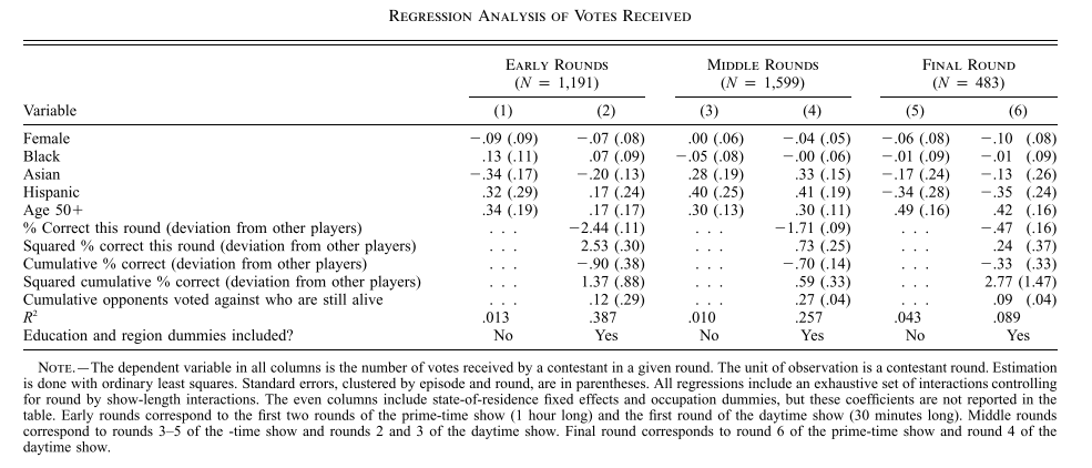
In a proverbial nutshell, the numbers not in parentheses indicate the sign and size of a given variable’s effect on receiving votes (in favor of being removed from the group). The numbers in parentheses are called “standard errors” (SE). They are strictly positive numbers. Roughly speaking, the smaller an SE relative to the magnitude of its corresponding variable’s effect on votes received, the more “statistically significant” is the effect. For example, consider the effect of being female in the game’s early rounds. Although this effect is negative (-0.09), because the magnitude is very close (in this case exactly equal) to its corresponding SE of 0.09, we say that the ‘female effect’ is non-existent in a statistical sense.^[1]

Taste-based discrimination is evident when an effect is positive and statistically significant in both the early and later rounds. Especially in the early rounds, votes should be based strictly on performance (i.e., a contestant’s ability to answer questions correctly on behalf of the group), not gender, ethnicity, or age. We see from column (1) that solely older contestants (age 50+) satisfy this condition (in column (1) the Age 50+ value of 0.34 is almost double the size of its corresponding SE of 0.19).^[2] Results in columns (3) and (4) for Age 50+ suggest a positive Age 50+ effect in the middle rounds as well.

Lastly, results for the variable “% Correct this round” provide evidence of the previous claims that contestants vote strategically in the early rounds of the contest but not in the later rounds. The large negative (and statistically significant) effect in column (2) of -2.44 indicates that, all else equal, contestants cast fewer votes for fellow contestants who provide correct answers more often. In the middle and final rounds, this effect should become positive if contestants vote strategically. We see from columns (4) and (6) that this does not happen—large negative (and statistically significant) effects persist in these later rounds.

Discrimination in Peer-to-Peer Lending

Pope and Sydnor (2011) also test for discrimination in a novel context—peer-to-peer lending on the website Prosper.com. Peer-to-peer lending is an alternative credit market that aggregates small amounts of money provided by individual lenders to fund moderately sized, uncollateralized loans to individual borrowers. Like most standard credit applications, Prosper.com publicizes loan information from the prospective borrower’s credit profile. However, borrowers may also include optional personal information in their listing in the form of photographs and text descriptions. These pictures and descriptions can provide potential lenders with signals about characteristics such as race, age, and gender that anti-discrimination laws typically prevent traditional lending institutions from using.

Using data from 110,000 loan listings appearing on Prosper.com from 2006-2007, the authors find evidence of significant racial discrimination in this market. Loan listings that include a photograph of a Black borrower result in a 30% reduction in the likelihood of that loan receiving funding, all else equal. Further, a loan listing tied to a Black borrower results in an interest rate that is 60 basis points higher than an equivalent listing for a white borrower.^[3] These results meet what the authors claim is a necessary condition for taste-based discrimination as defined by Levitt (2004). The question of whether the sufficient condition for this type of discrimination is met depends upon whether Black borrowers have statistically lower loan default rates and produce higher net returns for lenders. If the answer is “yes,” then together with the fact that they are less likely to receive funding and pay higher interest rates on loans they do receive, evidence of taste-based discrimination against Black borrowers is evinced.^[4]

The authors find that Black borrowers are approximately 36% more likely to default on their loans than are Whites with similar characteristics, and a lender’s average net return from a loan to a Black borrower is eight percentage points lower over a three-year period. Thus, they conclude that discrimination in peer-to-peer lending could in fact be information- rather than taste-based.

What’s In a Name?

According to the Economic Policy Institute’s (EPI’s) recent assessment of the US labor market, Black workers are twice as likely to be unemployed as White workers overall (6.4% vs. 3.1% unemployment rates, respectively)—a gap that, while narrower, persists among workers Black versus White workers with college degrees (3.5% vs. 2.2%) (Williams and Wilson, 2019). Further, when employed, Black workers with college or advanced degrees are more likely than their White counterparts to be underemployed—roughly 40% of Black college graduates are in jobs that typically do not require a college degree, compared with only 31% of their White counterparts. The EPI concludes that persistence in relatively high Black unemployment and skills-based underemployment indicates that racial discrimination remains a failure of the US labor market, even when the market is tight.

The question naturally arises as to whether employers do in fact favor White applicants over similarly skilled Black applicants (i.e. do employers discriminate among job candidates based upon race?). Bertrand and Mullainathan (2004) provide an answer based upon an intriguing field experiment where fictitious resumes were sent by the authors in response to help-wanted ads in Boston and Chicago newspapers. To manipulate perceived race, the resumes were randomly assigned Black- or White-sounding names, such as Lakisha Washington or Jamal Jones (Black-sounding names) in response to half the ads, and Emily Walsh or Greg Baker (White-sounding names) in response to the other half.

Because they were also interested in how credentials affect the racial gap in interview callbacks, Bertrand and Mullainathan (2004) varied the quality of the resumes. Higher-quality applicants had on average more labor-market experience and fewer holes in their employment history. These applicants were also more likely to have an email address, have completed some certification degree, possess foreign language skills, or have been awarded some honors. The authors generally sent four resumes in response to each ad—two higher-quality and two lower-quality. They randomly assigned Black-sounding names to one of the higher- and one of the lower-quality resumes. In total, the authors responded to over 1,300 employment ads in the sales, administrative support, clerical, and customer services job categories, sending out nearly 5,000 resumes in total.

Overall, White names received 50% more callbacks for interviews, which Bertrand and Mullainathan (2004) translate into a White name being as valuable as an additional eight years of experience on a Black person’s resume. Callbacks were also more responsive to resume quality for White than for Black names. The racial gap in interview callbacks was uniform across occupation, industry, and employer size. The authors also found that living in a “better” neighborhood (wealthier or more-educated or Whiter) increased callback rates. However, Blacks were not helped more than Whites by living in better neighborhoods. As the authors point out, if ghettos and bad neighborhoods are particularly stigmatizing for Blacks, one might have expected Blacks to have been helped more by having a better address. These results do not support this hypothesis.

Bertrand and Mullainathan (2004) also find that, across all sent resumes, the difference in percent callbacks for White- versus Black-sounding names is a statistically significant 3.2%. Callback discrimination based upon race occurs against both men and women, and the discrimination against Black women occurs mostly in conjunction with administrative rather than sales jobs.^[5]

It is humbling to think that Homo economicus employers, whose color-blindness is a patent feature of their rational minds, would not fall victim to racial discrimination in the hiring process. Thankfully, as the topic below, Awareness Reduces Racial Discrimination, suggests, when racial discrimination is brought to light its practice tends to dissipate.

Can Looks Deceive?

Similar to Prosper.com, but with a bit more (how shall we say?) gravity, online dating services create a natural setting within which to assess the impacts of a person’s physical appearance on a transaction between that person and a potential (how shall we say?) customer. One dating site, OkCupid, recently became interested in answering the simple question, to what extent do looks deceive? The site’s answer is based upon a natural experiment conducted with their users on what OkCupid named “Love is Blind Day,” January 15, 2013, celebrating the release of their new phone app. Comparing that day’s messaging data to the average day’s historically, Rudder (2014) uncovered several interesting (how shall we say?) relationships in the data.

For example, OkCupid’s site metrics (number of new conversations started per hour) were far beneath a typical Tuesday’s during the peak hours of 9 a.m. to 4 p.m. It seems that without the ability to view a prospective date’s photo, users were less motivated to make an initial inquiry. Nevertheless, Rudder reports that the conversations initiated during these seven hours without photos went deeper and contact details (e.g., email addresses and phone numbers) were exchanged more quickly. Sadly though, when the photos were restored at 4 p.m. sharp, the 2,200 users who were in the middle of their conversations that had started “blind” dissipated. As Rudder puts it, restoration of the photos was like turning on the bright lights at the bar at midnight. Conversations that had consisted of two messages prior to the 4 p.m. bewitching hour witnessed the largest drop relative to normal.

Curious about the extent to which a person’s photo matters on OkCupid, Rudder performed a simple test based upon a randomly chosen subsample of users. Half of the time their pages were accessed by a prospective suitor, their profiles were kept hidden. And half of the time the profiles were not hidden. This generated two independent sets of ratings for each member of the sample—one rating when the picture and profile text were presented together, the other for when the picture was presented alone. Rudder found a strong positive correlation between the ratings with and without the profile text included, suggesting that a picture really is worth a thousand words. A person’s rating was driven by the appeal of their picture rather than their profile. To put it less sanguinely, we Homo sapiens tend to be superficial when it comes to choosing our dating partners.^[6]

The Spillover of Racialization

To what extent might racial prejudice spill over into (i.e., infect) opinions about public policy, such as health care and fiscal stimulus? The election of Barack Obama in 2008 as the 44th President of the United States helps provide an answer. Using data from a nationally representative survey experiment, Tesler (2012) documents the impact of race and racial attitudes on opinions concerning national healthcare policy before and after Obama’s election. The authors find that racial attitudes were both an important determinant of White Americans’ opinions about healthcare policy in the fall of 2009 and that the influence of these attitudes increased significantly after President Obama became the face of the policy. Results from the experiment show that racial attitudes had a significantly greater impact on healthcare opinions when framed as part of President Obama’s plan than they had when the same policies were attributed to President Clinton’s 1993 healthcare initiative. In other words, Tesler uncovers what he calls a spillover of racialization, which situates Obama’s race—and the public’s race-based reactions to him—as the primary reason why public opinion about national healthcare policy racialized in the fall of 2009.

As Tesler points out, spillover of racialization—whereby racial attitudes have a bearing on political preferences—is rather straightforward for race-targeted public policies such as affirmative action and federal aid to minorities. These types of issues are thought to readily evoke racial predispositions since a natural associative link exists between policy substance and feelings toward the groups who benefit from them. However, this link is not as readily apparent for broader issues such as healthcare and fiscal stimulus.

Tesler further avers that, after receiving little media attention during the first half of 2009, the debate over healthcare reform became one of the most reported news stories in America from early July through the remainder of the calendar year, so much so that roughly half of Americans reported following the healthcare reform debate very closely in 2009 (Pew Research Center, 2009). If, as the spillover of racialization hypothesis contends, Obama’s connection to the issue helped racialize their policy preferences, then the effect of racial attitudes on White Americans’ opinions should have increased from before to after his healthcare reform plan was subjected to such intense media scrutiny.

Tesler utilizes observational data from repeated cross-sectional surveys conducted by the American National Election Study (ANES). The ANES healthcare question asks respondents to place themselves on a seven-point government-to-private insurance preference scale. To obtain corresponding information on racial resentment, Tesler re-interviewed individuals who had participated in the ANES survey both before and after President Obama’s election. The author argues that his racial-resentment measure taps into subtle hostility among White Americans toward Black Americans. The measure is based upon four questions about Black work ethic, the impact of discrimination on Black American advancement, and notions of Black people getting more than they deserve—themes thought to undergird a symbolic racialism belief system—and coalesced into a seven-point scale from low to high levels of racial resentment.

Tesler finds that, for White respondents, moving from those harboring the least amount of racial resentment to those harboring the most resentment increased the proportion of those saying that the national healthcare system should be left up to individuals by approximately 30 percentage points (from 10% to 40%) in December 2007, when President Clinton was the face of national healthcare policy. However, the same change in these individuals’ resentment levels (i.e., again moving from those White respondents harboring the least amount of racial resentment to those harboring the most resentment) increased their support for private insurance by roughly 60 percentage points (from 10% to 70%) in November 2009, when President Obama served as the face of the same national healthcare policy—a statistically significant difference. This leads Tesler to conclude that with the election of President Obama racial attitudes became more important in White Americans’ beliefs about healthcare relative to nonracial considerations like partisanship and ideology.

In an additional experiment, Tesler investigated opinions regarding the $787 billion economic stimulus package passed by Congress in 2009. Respondents were divided into two subsets. In one subset, respondents were asked if they thought the stimulus package approved by congressional Democrats was a good or bad idea, the other was asked the same question but with approval instead being granted by President Obama. The author finds that moving from least to most racial resentment decreased the proportion of White respondents saying that the stimulus program was a good idea by less than 10 percentage points when congressional Democrats are identified as the approving authority, but by approximately 70 percentage points when President Obama is identified as the approving authority. In other words, the incidence of racialization spillover is even more profound than it was regarding national healthcare policy.

Awareness Reduces Racial Discrimination

In situations where racial discrimination is known to exist, does informing the public of its existence encourage perpetrators to repudiate its practice? Pope et al. (2018) devised a novel approach to answer this question. In 2003, the authors began by analyzing data from the National Basketball Association (NBA) for the years 1991-2003. They found that White and Black players received relatively fewer personal fouls when more of the referees officiating the game were of their own race. This in-group favoritism (or, alternatively stated, out-group racial bias) displayed by NBA referees was large enough to influence game outcomes.

In May of 2007, the results of this study received widespread media attention—front-page coverage in the New York Times and many other newspapers, and extensive coverage on major news networks, ESPN, and talk radio. Subsequently, the authors analyzed NBA data for the years 2007–2010 and found an absence of this out-group racial bias, although other biases were found to persist (e.g., referees tend to favor the home team, the team that is losing in a given game, and teams that are losing the game count in a playoff setting).

The table below contains Pope et al.’s (2018) specific findings:

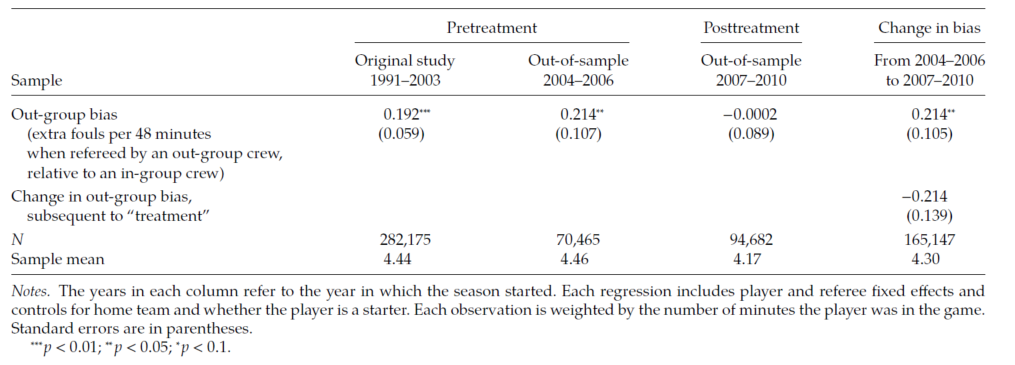
Similar to the presentation of Levitt’s (2004) results (see Discrimination in The Weakest Link Game Show above), marginal effects are presented with their corresponding standard errors in parentheses. Pope et al. provide additional notation to distinguish statistically significant effects from those that are not—superscripts with more asterisks indicate more statistical significance; those effects without any asterisks indicate no statistical significance. The marginal effects in the pretreatment period—based upon data from the original study and an additional study covering the years 2004-2006—are positive and statistically significant (0.192 and 0.214, respectively), leading the authors to conclude that, prior to media attention, significantly more fouls were called on Black players when the referee crew was predominantly White. In the post-treatment period—based upon data from 2007-2010—the marginal effect is not statistically significant (i.e., no effect exists). Hence, the prior racial bias among referee crews in the NBA dissipated after having received widespread media attention. That’s a slam dunk for the NBA and another one for Homo sapiens in general! Raising awareness of racial discrimination, especially when we can quantify its presence, serves as a nudge toward racial equality.

Improving Student Performance

Levitt et al. (2016) designed a field experiment to test the effects of different incentive mechanisms on the academic performance of students in low-performing elementary, middle, and high schools in the Chicago public school system and, in the process, test for the existence of loss aversion and time inconsistency among the students. Students were offered one of the following rewards for improving upon a previous (baseline) computerized reading or math test: $10 in cash (“financial low”), $20 in cash (“financial high”), or a trophy and posting of a student’s photograph in the school’s entrance (“nonfinancial”).

To test for loss aversion among the students, financial and non-financial rewards were delivered in one of two ways: (1) the test administrator held up the $10 bill, $20 bill, or trophy at the front of the room before the test began (the authors call this the “gain condition”), or (2) students received the $10 bill, $20 bill, or trophy at the start of the testing session and were informed that they would keep the reward if their performance improved and lose the reward if it did not (“loss condition”). The following results were obtained:^[7],^[8]

1. The $20 incentive (framed either as a gain or loss) delivered immediately after students completed the test increased the average student’s test score. The $10 incentive did not increase the average student’s test score and even lowered performance on future tests.
2. The trophy delivered immediately after the test increased the average student’s test score less dramatically than the $20 incentive. Scores increased most dramatically for younger students who received trophies.
3. The average student’s test score increased more in the loss condition than in the gain condition, but the difference is not statistically significant. Hence, the average student does not exhibit loss aversion with respect to how the reward for improved performance is distributed.
4. Delayed rewards (delivered one month after completion of the exam rather than immediately) did not increase the average student’s test score. This suggests the existence of hyperbolic discounting, where rewards delayed in the near term are discounted at an excessively high rate (recall our earlier exploration of this phenomenon in Chapter 4).
5. Overall, math scores increased more than reading scores across all students. Boys increased their scores in these subjects more than girls.

Improving Teacher Performance

Fryer et al. (2022) demonstrate that, unlike Levitt et al.’s (2016) findings for elementary and middle school students in Chicago, exploiting the power of loss aversion—where the student’s teachers are paid at the beginning of the school year and asked to give back the money if their students do not improve sufficiently (loss treatment)—leads to statistically significant increases in their students’ math test scores. A second treatment identical to the loss treatment but with year-end bonuses linked to student performance (gain treatment) yields smaller and statistically insignificant results. The authors conclude that because teachers exhibit loss aversion (in terms of rewards tied to their students’ academic performance), a loss-treatment approach is the most effective way to incentivize teachers to improve student performance.

In specific, Fryer et al. find that, all else equal, the average student who was taught by a teacher who had been randomly assigned to the loss treatment gained (statistically significant) percentile-ranking points relative to her nine nearest students during the math exam; gains that persisted in time after the treatment. Students who were taught by teachers who were randomly assigned to the gain treatment showed markedly lower and statistically insignificant gains. Therefore, it seems as though a teacher’s performance can be more effectively nudged by appealing to his sense of loss aversion rather than merely the teacher’s desire for gain.

Healthcare Report Cards

Recall from Chapter 8 the simultaneous-move game where provisioning one of two players with additional information actually perversely affected the game’s analytical equilibrium. The message was clear. The rational choice model’s tenet that more information leads to improved performance is not universal. Especially when it comes to the experience of Homo sapiens, situations where the provision of additional information leads to a perverse outcome are not necessarily in short supply.

Dranove et al. (2003) provide a seminal example with their study of Healthcare Report Cards—public disclosure of patient health outcomes at the level of the individual physician or hospital or both—that are intended to improve the performance of healthcare providers. In their study, the authors analyzed New York’s and Pennsylvania’s publications of physician and hospital coronary artery bypass graft (CABG) surgery mortality rates in the 1990s. At the time, the merits of these types of report cards were in much debate. Supporters argued that report cards enable patients to identify the best physicians and hospitals while simultaneously giving healthcare providers powerful incentives to improve quality. Skeptics countered that report cards encourage providers to “game” the system by avoiding sick patients and/or seeking healthy patients.

As Dranove et al. point out, low-quality providers have strong incentives to avoid the sick and seek the healthy under this type of reporting system. By shifting their practice toward healthier patients, inferior providers make it difficult for report cards to distinguish them from their higher-quality counterparts because relatively healthy patients have higher likelihoods of better outcomes regardless of provider. As the authors put it, low-quality providers can therefore pool with their high-quality counterparts, making it more difficult for the report cards to distinguish between the two.

Spoiler alert: The authors find that while the report card system increased the quantity of CABG surgeries among patients suffering from acute myocardial infarction (AMI) (i.e., heart attacks), it changed the surgery’s incidence from sicker AMI patients toward healthier AMI patients. Overall, this led to higher costs and deterioration of outcomes, especially among the sicker AMI patients (i.e., the report cards were welfare-reducing).

Dranove et al. find that the introduction of report cards increased the probability that the average AMI patient would undergo CABG surgery within one year of hospital admission by between 0.60 to 0.91 percentage points. As the authors point out, these report-card effects are considerable, given that the probability of CABG within one year for an elderly AMI patient during their sample period was approximately 13%. However, the report-card effects did not occur immediately (i.e., within one day of admission to the hospital). Indeed, the immediate report-card effect is estimated to have been negative for the average AMI patient (ranging from -0.59 to -0.78 percentage points). The authors also find evidence to suggest that the report card system led to sicker patients being less likely to undergo CABG surgery within one year of admission. Report-card effects on average (1) led to increases in total hospital expenditures in the year after admission of an AMI patient, (2) provided some evidence of increased patient readmission with heart failure within one year, and (3) provided some evidence of increases in mortality within one year of admission. These perverse welfare effects were particularly strong among sicker AMI patients.

This is one of several examples in the empirical literature of perverse outcomes associated with what, on the surface, would seem to be naturally beneficial incentives, or nudges, meant to improve the social welfare of Homo sapiens, in this case with respect to health care.

Losing Can Lead to Winning

Berger and Pope (2011) conducted another study using data from the NBA, this time seeking to determine if teams who, going into halftime of a typical game and down a certain number of points, collectively exhibit loss aversion—in terms of not wanting to lose the game—by winning the game in the end. In other words, do NBA players demonstrate loss aversion collectively as a team?

The authors analyzed more than 18,000 NBA games played from 1993-2009 and found that teams behind by one point at halftime win more often than teams ahead at halftime by one point—approximately 6% more often than expected. This finding suggests the presence of (1) loss aversion—being behind at halftime motivates a team not to lose more than being ahead at halftime motivates a team to win, (2) diminishing sensitivity—the losing team cannot be too far behind at halftime, and (3) reference dependence—being behind at halftime helps the losing team establish the goal of winning.^[9]

The graph below depicts Berger and Pope’s results:

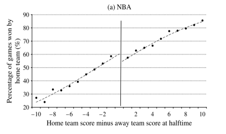
The upward slope of the hashed line indicates that the more points the home team has at halftime relative to the away team, the more likely the home team will wind up winning the game. The line’s discontinuity in the neighborhood of zero depicts the study’s main results. At one point behind, the probability of the home team winning is roughly 60%. At one point ahead, the home team’s probability of winning drops to roughly 54%, which is slightly higher than if the home team is down by two points at halftime. Similarly, if the home team is ahead by two points at halftime, then its probability of winning is over 60%. Hence, when two teams are within a few points of each other going into halftime, halftime is indeed a game’s reference point. And the home team’s chances of winning the game diminishes fairly rapidly as it falls further behind going into halftime. This latter result can be taken as evidence that a home team’s collective marginal disutility of losing diminishes in concert with its chances of winning. Berger and Pope also find that, all else equal, when the home team is losing at halftime, its probability of winning the game increases by anywhere from 6% to 8%.

Loss Aversion in Professional Golf

Professional basketball is not the only sport lending itself to empirical testing of behavioral economics’ preeminent theories. Professional golf is also amenable. Using data on over 2.5 million putts measured by laser technology, Pope and Schweitzer (2011) test for the presence of loss aversion among professional golfers competing on the Professional Golf Association (PGA) Tour. As the authors point out, golf provides a natural setting to test for loss aversion because golfers are rewarded for the total number of strokes they take during a tournament, yet each individual hole has a salient reference point, par.

Pope and Schweitzer find that when golfers are “under par” (e.g., putting for a “birdie” that would earn them a score one stroke under par), they are 2% less likely to make the putt than when they are putting for par or are “over par” (e.g., putting for a “bogey” that would earn them one stroke over par). Even the best golfers—including Tiger Woods at the time—show evidence of loss aversion in these situations. Loss aversion motivates golfers to make a higher percentage of puts when they are putting for a bogey than a birdie.

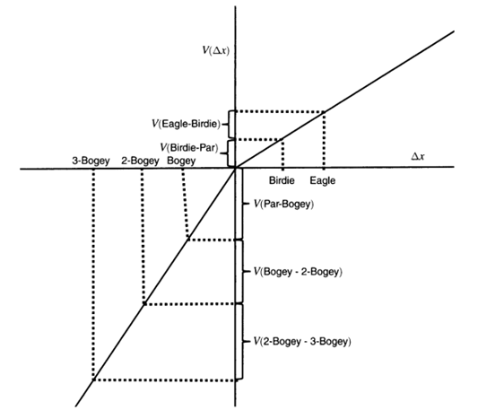
Two figures coalesce the authors’ econometric results. The first figure represents the typical golfer’s value function. Note the function’s reference point (i.e., its origin) at par. The steeper portion of the function defined over the disutility region is associated with missing par and thus bogeying a putt (one-over-par is a bogey, two-over-par is a double bogey, and so on). The flatter portion of the function defined over the utility region corresponds to scoring under par with a birdie (one under par), eagle (two under par), or albatross (greater than two under par). Recall that the relative steepness of the function in the disutility region depicts loss aversion. The linearity of the function indicates an absence of the diminishing effect.

The next figure depicts the relationships between the average golfer’s fraction of putts made when putting for par and for birdie, respectively, relative to distance from the hole. As expected, regardless of whether a golfer is putting for birdie or par, the fraction of putts made decreases as the distance to the hole increases. Of particular interest in this study is that, at each distance, the fraction of putts made is less when the golfer is putting for birdie as opposed to par—again, evidence of loss aversion.

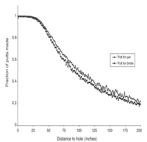
To reiterate, this study’s main econometric results reveal a negative effect on sinking a putt when the typical golfer is putting for birdie, and a positive effect on putting for bogey. Consistent with the previous graphs, these numerical results suggest that the typical professional golfer is more likely to sink a put for bogey and less likely to sink the putt for birdie (i.e., the typical golfer is indeed loss averse).^[10]

Are Cigarette Smokers Hyperbolic Time Discounters?

Recall from Chapter 4 the distinction between time-consistent exponential time discounters (Homo economicus) and potentially time-inconsistent hyperbolic discounters (Homo sapiens). The discounting time paths for exponential versus hyperbolic discounting looked like this:

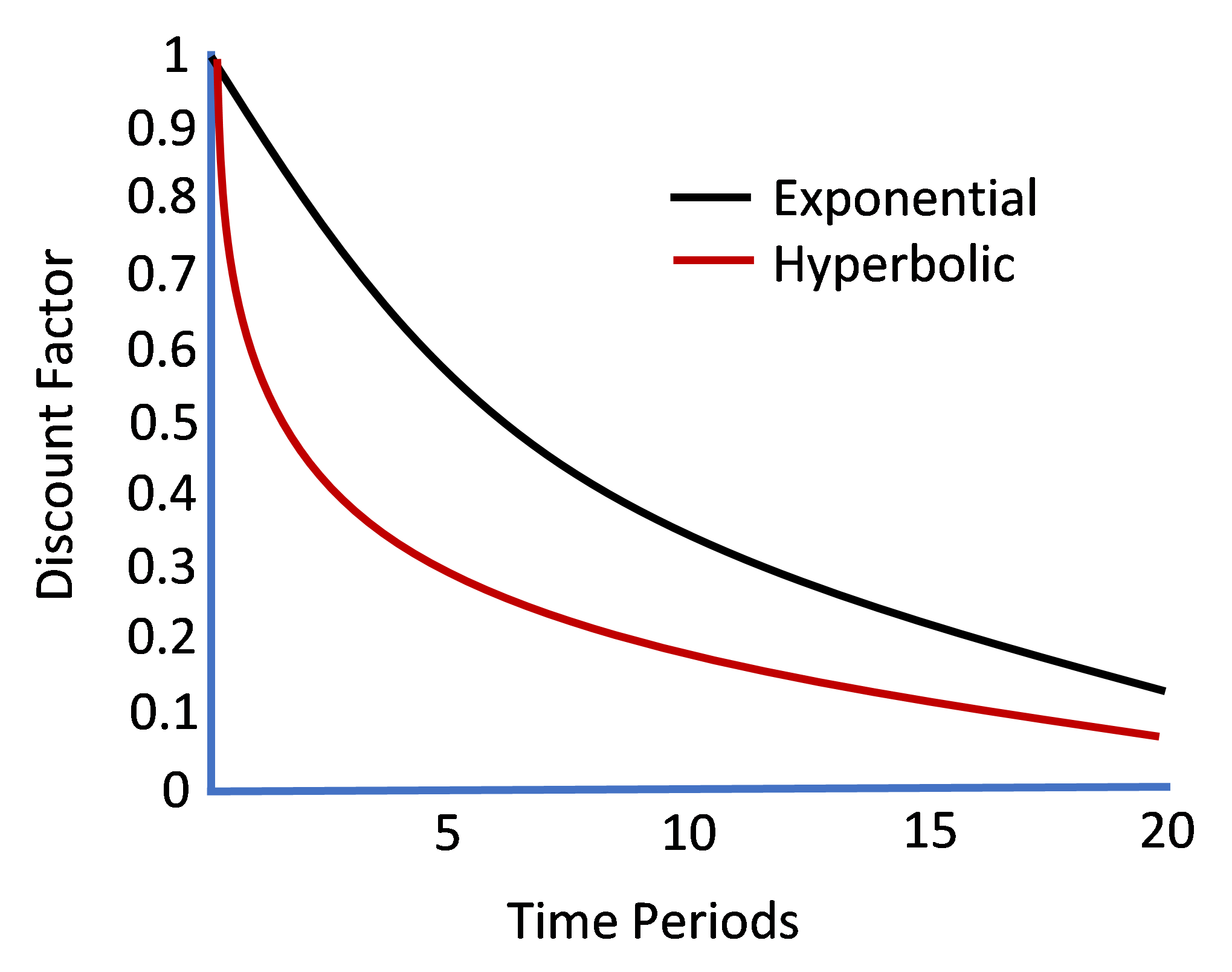
A feature distinguishing a hyperbolic from an exponential time discounter is that the former discounts time delays in near-future consumption at much higher rates than the latter, but the discounting of more distant-future consumption converges between the two.

In contrast with Becker and Murphy’s (1988) early theoretical work explaining rational addiction among Homo economicus based upon exponential time discounting, experimental research aimed at explaining addiction among Homo sapiens has found that hyperbolic discounting of future consumption can at least partially explain the impulsive behavior exhibited by those among us with addictions to drugs such as alcohol, heroin, and opioids (c.f., Vuchinich and Simpson, 1998 and Madden et al., 1997).^[11] Bickel et al. (1999) also find evidence of hyperbolic time discounting among cigarette smokers. In their field experiment, the authors compare the discounting of hypothetical monetary payments by current and ex-smokers of cigarettes, as well as those who have never smoked (henceforth “never smokers”). For current smokers, the authors also examine discounting behavior associated with delayed hypothetical payment in cigarettes.^[12], ^[13]

The authors find that current smokers discount the value of a delayed monetary payment more than ex- and never-smokers (the latter two groups do not differ in their discounting behaviors). For current smokers, delayed payment in cigarettes loses subjective value more rapidly than delayed monetary payment. The hyperbolic equation provides a better fit of the data for cigarette smokers than the exponential equation for 74 out of the 89 different comparisons between current cigarette smokers, on the one hand, and ex- and never-smokers on the other. Bickel et al. (1999) conclude that cigarette smoking, like other forms of drug dependence, is characterized by rapid loss of subjective value for delayed outcomes (i.e., pronounced hyperbolic discounting).

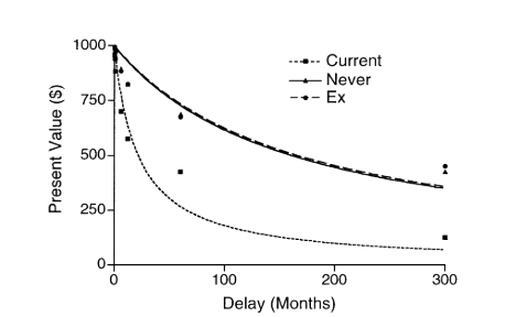
The figure below shows Bickel et al.’s results for a monetary payment scheme. The curves represent the median indifference points (i.e., the estimated values of immediate payment at the respective points of subjective equality with each of seven different delay periods) for current smokers, never-smokers, and ex-smokers. We see that the subjective values decrease more rapidly for smokers (along the curve resembling a hyperbolic discounting function) than for never-smokers and ex-smokers (along curves resembling exponential discounting functions). For example, for smokers, a $1000 payment lost 42.5% of its value when delayed by one year, but for never- and ex-smokers, a $1000 payment lost only 17.5% of its value when delayed by one year.

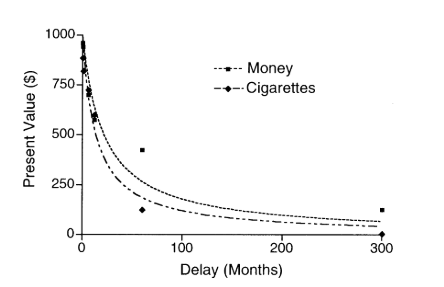
As the figure below shows, the bulge in current smokers’ hyperbolic discounting function is more pronounced for the cigarette payment scheme (the curve associated with the monetary payment scheme is reproduced from the previous figure for ease of comparison).

Arrest Rates and Crime Reduction

As Levitt (1998) points out, the linchpin of the rational-choice model of crime is the concept of deterrence: criminal Homo economicus will choose to commit fewer criminal acts when faced with higher probabilities of detection or more severe sanctions. Levitt conjectures that criminal Homo sapiens may defy this rational-choice model of deterrence by being poorly informed about the likelihood of getting caught, over-optimism about their abilities to evade detection, myopia due to the time gap between committing the crime and imprisonment, or perhaps because serving a prison sentence satisfies a rite of passage among a criminal’s peers.

Levitt further points out that empirically testing for a deterrence effect among would-be criminals is fraught with challenges because increasing the expected punishment associated with a given crime can potentially reduce crime through two different channels. The first channel is deterrence—larger penalties and/or higher arrest rates induce criminals to commit fewer crimes. The second channel is incapacitation—if criminals commit multiple offenses and punishment takes the form of imprisonment, increasing expected punishment will also reduce crime by getting criminals off the streets. While a criminal is imprisoned, he is unable to engage in criminal actions that otherwise would have taken place, which biases the statistical effect of deterrence upward (i.e., due to the incapacitation effect, an increase in deterrence measures undertaken by the police would be identified as having a larger negative impact on crime reduction than is truly the case).

Levitt utilized annual reported-crime data from the Federal Bureau of Investigation (FBI) for 59 of the largest U.S. cities over the period 1970-1992 to test for a deterrence effect driven by changes in arrest rates. His results suggest that (1) incapacitation predominately reduces the incidence of rape, (2) incapacitation and deterrence effects are of equal magnitude in reducing the incidence of robbery, and (3) the deterrence effect outweighs the incapacitation effect in reducing aggravated assault and property crimes (Levitt estimates that the deterrence effect accounts for more than 75% of the observed effect of arrest rates on property crime).

Hence, when it comes to arrest rates, criminal Homo economicus and Homo sapiens share similar responses to deterrence.

Interpersonal Dynamics in a Simulated Prison

There is substantial evidence that prisons in the US (if not worldwide) neither rehabilitate prisoners nor deter future crime. In its most recent report on recidivism in the US, the US Justice Department reports that 44% of state prisoners released in 2005 across 30 states were re-arrested within one year of their release, 68% within four years, 79% within six years, and 83% within nine years (Alper et al., 2018). Of released drug offenders, 77% were re-arrested for a non-drug crime within nine years after release. During each year, and cumulatively during the nine-year follow-up period, released non-violent offenders were more likely than released violent offenders to be arrested again (Alper et al., 2018).

Haney et al. (1973) pose (and then seek to answer) a nagging question pertaining to what lies behind these statistics. To what extent can the deplorable conditions of our penal system and their often-dehumanizing effects upon prisoners and guards—conditions that likely contribute to recidivism—be explained by the nature of the people who administer it (prison guards) and the nature of the people who populate it (prisoners)? The authors’ dispositional hypothesis is that a major contributing cause of these conditions can indeed be traced to some innate or acquired characteristics of the correctional and inmate populations. As the authors point out, the hypothesis has been embraced by both the proponents of the prison status quo, who blame the nature of prisoners for these conditions, as well as the status quo’s critics, who blame the motives and personality structures of guards and staff.

To understand the genesis of prison culture—in particular, the cultural effect on the disposition of both prisoners and guards—Haney et al. (1973) undertook one of the most notorious (or, depending upon one’s perspective, noteworthy) field experiments ever conducted with willing, non-incarcerated adults. The authors designed a functional simulation of a US prison in which subjects who were drawn from a homogeneous, “normal” sample of male college students role-played prisoners and guards for an extended period of time. Half the subjects were randomly assigned to the prisoner group, which was incarcerated for nearly one full week. The other half were randomly assigned to the prison guard group, which played its role for eight hours each day. The behaviors of both groups were observed, recorded, and analyzed by the authors, particularly regarding transactions occurring between and within each group of subjects.

The 21 subjects who ultimately participated in the experiment (out of a total of 75 applicants) were judged to be the most physically and emotionally stable, most mature, and exhibited the least anti-social behavior. The prison was constructed in a basement corridor in the Psychology Department’s building at Stanford University. It consisted of three small cells (6’ x 9’), each cell housing three prisoners. A cot, mattress, sheet, and pillow for each prisoner were the only pieces of furniture in each cell. A small, unlit closet across from the cells (2’ x 2’ x 7’) served as a solitary confinement facility. Several rooms in an adjacent facility were used as guards’ rooms and quarters for a “warden” and “superintendent.” The prisoners were each issued identical, ill-fitting, prisoner uniforms to instill uniformity and anonymity in the prisoners’ daily existence. The guards’ uniforms consisted of a plain khaki shirt and trousers, a whistle, wooden baton, and reflecting sunglasses that made eye contact impossible.

With help from the Palo Alto City Police Department, the prisoners were each “arrested” (with handcuffs, no less) at their residences under suspicion of burglary and armed robbery, taken to the police station, and “processed” under normal induction procedures. Once they arrived at the simulated prison (blindfolded, no less), they continued with standard induction procedures, which included being stripped naked, sprayed with a deodorant, and made to stand alone naked in a prison yard for a short period of time. Each prisoner was then put in his cell and ordered to remain silent. During their confinement, the prisoners were fed three meals a day, allowed three supervised toilet visits, and were allotted two hours daily for the privilege of reading and letter-writing.

Data was gathered via videotaping, audio recordings, personal observations, and a variety of checklists filled out by the guards and researchers. Through subsequent analysis of the data, Haney et al. (1973) found that the personal behaviors of the prisoners and guards, and the social interactions between them, supported many commonly held conceptions of prison life and validated anecdotal evidence provided by real-life ex-convicts. In general, both prisoners and guards tended toward increased negativity over the week in terms of their dispositions. For both prisoners and guards, self-evaluations became more disapproving as their experiences were internalized. Prisoners generally adopted a passive response mode while guards assumed active, initiating roles in all prisoner-guard interactions.^[14]

Specifically, Haney et al. found that the extent to which a prisoner scored high on his personality test for rigidity, adherence to conventional values, and acceptance of authority helped determine the likelihood that he adjusted more effectively to the authoritarian prison environment. In written self-reports, prisoners expressed nearly three times as much negativity as positivity. Guards expressed slightly more negativity than positivity. Prisoners also showed roughly three times as much mood fluctuation as did the guards.

Haney et al. conclude:

“The conferring of differential power on the status of “guard” and “prisoner” constituted, in effect, the institutional validation of those roles. But further, many of the subjects ceased distinguishing between prison role and their prior self-identities. When this occurred, within what was a surprisingly short period of time, we witnessed a sample of normal, healthy American college students fractionate into a group of prison guards who seemed to derive pleasure from insulting, threatening, humiliating, and dehumanizing their peers—those who by chance selection had been assigned to the prisoner role. The typical prisoner syndrome was one of passivity, dependency, depression, helplessness and self-deprecation.” (p. 89)

For those of us who are skeptical of the simulated nature of this experiment’s constructed prison environment, Haney et al. offer this final thought:

“In one sense, the profound psychological effects we observed under relatively minimal prison-like conditions which existed in our mock prison make the results even more significant and force us to wonder about the devastating impact of chronic incarceration in real prisons.” (p. 91)

At the very least, this experiment demonstrates how manipulatable and culpable Homo sapiens can become in the context of a field experiment.^[15]

Corruption in Sumo Wrestling

In one of their most well-known studies, Duggan and Levitt (2002) uncovered the extent of corruption in Japan’s national sport, sumo wrestling. To understand how they did so, one must know something about how sumo wrestling tournaments work.

A sumo tournament involves 66 wrestlers (rikishi) competing in 15 bouts each. A wrestler who achieves a winning record (eight wins or more) in a tournament is guaranteed to rise in the official ranking of the nation’s wrestlers. A wrestler with a losing record in the tournament (seven wins or less) falls in the national rankings. A wrestler’s ranking is a source of prestige and the basis for salary determination and various in-kind perks.

As Duggan and Levitt point out, the key institutional feature of sumo wrestling making it ripe for corruption is the concomitant nonlinearity in the ranking (and thus payoff) function for competitors, depicted in the figure below:

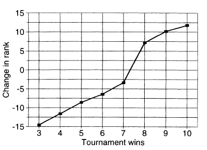
We see that a wrestler who achieves a losing record of seven wins and eight losses (7-8) can expect to drop in the rankings by roughly three places (e.g., if, going into the tournament, the wrestler was ranked third nationally, after the tournament, he is now ranked sixth). To the contrary, a wrestler achieving a winning record of 8-7 in the tournament can expect to rise in rank by roughly eight places. Consequently, a wrestler entering the final match of a tournament with a 7-7 record has far more to gain from a victory than an opponent with a record of, say, 8-6 has to lose.

Following almost 300 wrestlers from 1989-2000, the authors find that wrestlers who are on the margin for attaining their eighth victory in a given tournament (in what’s known as a “bubble match”) win far more often than one would expect. Further, whereas the wrestler who is on the margin for his eighth victory in a bubble match wins with a surprisingly high frequency, the next time the same two wrestlers face each other in another tournament, it is the opponent (i.e., the wrestler who threw the bubble match) who has an unusually high win percentage. In other words, Duggan and Levitt not only uncover corruption in the bubble match itself but also corruption in the subsequent match between the same two wrestlers. This corruption comes in the form of the earlier bubble match’s winner duly compensating the loser by similarly throwing the current match.

Duggan and Levitt depict their finding in the figure below:

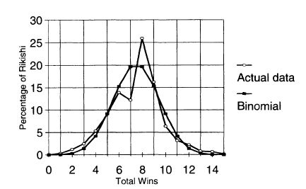
The figure shows two curves—one based on the actual data, the other based on the binomial distribution, which represents the distribution we would expect to hold between the wrestlers and their wins, all else equal. The binomial distribution depicts a nice, bell-shaped curve where the largest percentages of wrestlers win between 5 and 10 matches per tournament. The obvious spike in the actual data over eight wins, which is aligned with over 25% of the wrestlers when we would expect only 20%, suggests a preponderance of unexpected outcomes in bubble matches.

Interestingly, Duggan and Levitt find that the bubble match effect disappears in tournaments with high levels of media scrutiny and when the opponent (i.e., the wrestler who would otherwise agree to throw the bubble match) is in the running for one of the tournament’s special prizes.^[16] By contrast, success on the bubble increases for veteran wrestlers (i.e., all else equal, veterans are more likely to win bubble matches in tournaments where they go into the match with seven wins, seven losses).

Corruption in Emergency Ambulance Services

To improve emergency ambulance response times in England in the early 2000’s, authorities implemented a common response-time target for “ambulance trusts” (i.e., regional units) that 75% of potentially immediately life-threatening (Category A) emergency telephone calls be met within 8 minutes of the call having been placed. Less serious emergency calls (e.g., concerning serious but not life-threatening or neither serious nor life-threatening) were assigned less stringent targets. In addition, a “star rating system” was established rewarding or penalizing the trusts based upon the extent to which they met or did not meet the targets.

As Bevan and Hamblin (2009) point out, hospital rankings based upon the annual star ratings were easy to understand, and the results were widely disseminated (published in national and local newspapers and on websites, and featured on national and local television). Hospital staff was highly engaged with the information used to determine the ratings. Further, the star ratings mattered for chief executives, as being zero-rated resulted in damage to their professional reputations and affected staff recruitment. As a result, the star rating system was widely considered to be a salient mechanism for improving hospital performance and, as a result, was ripe for attempts by hospitals and ambulance trusts to manipulate it.

Bevan and Hamblin find that, on the surface, the implementation of Category A ambulance-service targets in 2002 had a noticeable impact on response times. The percentage of response times per trust meeting the eight-minute target increased markedly after 2002 and remained up in the range of 70%–90% meeting the target through the study period of 2005.

However, digging deeper into the data, Bevan and Hamblin uncovered pervasive evidence of cheating among the trusts. As the authors point out, the system’s intense focus on the Category A target gave rise to several concerns, among them the obvious incentive to classify calls as Categories B and C rather than Category A, and the fact that arriving at the scene in 8.01 minutes was now inevitably seen as a failure. Earlier investigations had concluded that the former concern—reduced number of calls classified as Category A—was not commonly practiced among the trusts. Not so the latter concern. Bevan and Hamblin find that among the trusts’ response times taking longer than the targeted eight minutes, roughly 30% had been ‘corrected’, i.e. re-recorded as having taken less than eight minutes.

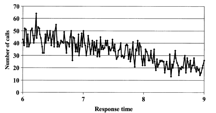
First, consider the recorded response-time data for a trust that exhibited an expected (‘uncorrected’) distribution of response times—a “noisy” decline in the number of responses with no obvious jump around the eight-minute threshold:

Next, consider data from two other trusts that exhibit what appear to be curious drops in reported response times at the 8-minute threshold:

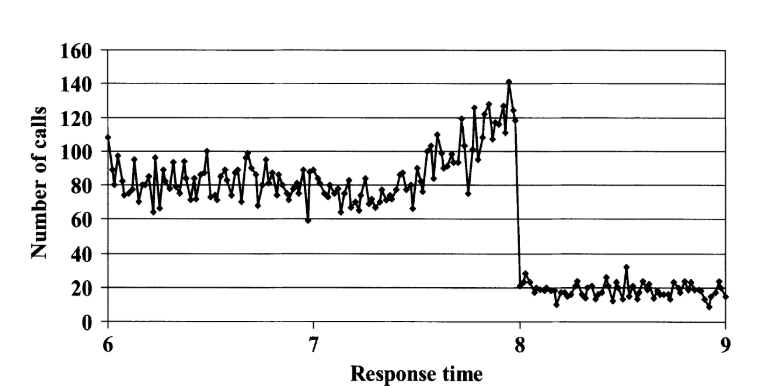
The drop in reported response times is obviously more marked in the bottom figure, but also present in the first of these two figures. Clearly, something suspicious occurred with the reporting for these two trusts. As with sumo wrestlers, the putative setting of a harmless rule induced perverse behavior among the targeted group of Homo sapiens. In the case of England’s emergency ambulance services, it appears that some of the ambulance trusts chose to disingenuously fudge their reported Category A response times.

New York City’s Taxi Cab Drivers

Camerer et al. (1997) clued into the fact that taxi cab drivers are an ideal population to study for unexpected labor market behavior because the structure of the taxi cab market (at least, New York City’s (NYC’s) market in the late 1980s and early 1990s) enabled drivers to choose how many hours to drive during a given shift. As a result, drivers faced wages that fluctuated daily due to “demand shocks” caused by weather, subway breakdowns, day-of-the-week effects (e.g., Mondays may generally be busier than Tuesdays each week), holidays, conventions, etc. Although rates per mile are set by law, on busy days, drivers may have spent less time searching for customers and thus, all else equal, earned a higher hourly wage. These hourly wages are transitory. They tend to be correlated within a given day and uncorrelated across different days. In other words, if today is a busy day for a driver, she can earn a relatively high hourly wage. But if the very next day is slow, then the driver will earn a relatively low hourly wage.

Camerer et al. compiled different samples of NYC taxi drivers over three different time periods: (1) from October 29th to November 5th, 1990, consisting of over 1000 trip sheets filled out by roughly 500 different drivers (henceforth the TLC1 sample), (2) from November 1st to November 3rd, 1988, consisting of over 700 trip sheets filled out by the same number of drivers (henceforth the TLC2 sample), and (3) during the spring of 1994, consisting of roughly 70 trip sheets filled out by 13 different drivers (henceforth the TRIP sample). For each sample, Camerer et al. divided drivers into low- and high-experience subsamples.

Generally speaking, the authors find that drivers (particularly inexperienced ones) made labor supply decisions “one day at a time” (i.e., framed narrowly) rather than inter-temporally substituting their labor and leisure hours across multiple days (i.e., framed broadly) in response to temporary hourly wage changes (as you’ve probably guessed already, Homo economicus drivers frame broadly). The typical (Homo sapiens) driver set a loose daily income target (which served as the driver’s reference point) and quit working once she reached that target (which resulted in a negative relationship between the number of hours she chose to work and the driver’s daily hourly wage rate). In other words, as the driver’s hourly wage rose, she chose to drive fewer hours—a perverse outcome in a rational-choice model of any type of worker’s behavior. As Camerer et al. point out, the driver’s reference point established a daily mental account and also suggests loss-averting behavior in the sense that, on a slow day, a driver chose to work more hours to reach the reference point, thus avoiding the “loss” that comes with under-performing on the job.

Specifically, the authors find that low-experienced drivers exhibit negative responses to wage increases in each sample, but the responses are statistically significant only in the TRIP sample and marginally significant in the TLC2 sample. High-experienced drivers exhibit a negative response solely in the TLC1 sample. Therefore, Camerer et al. find some evidence of reference dependency, mental accounting, and loss aversion among NYC’s famed taxi drivers.

Savings Plans for the Time-Inconsistent

Homo sapiens who are time inconsistent when it comes to saving income for future consumption are prone to save too little now for what they later realize they needed in order to maintain their standard of living. In response, two types of “tailored savings plans” have been developed over time, targeting segments of the population with historically low personal savings rates. One plan—Prize-Linked Savings Accounts (PLSAs)—encourages people to increase their savings rates by adding a lottery component to what is an otherwise traditional savings account at a participating bank (Morton, 2015). Depositors’ accounts are automatically entered into periodic drawings based upon their account balances during a given period. Depositors then have a chance to win prizes, which are funded through the interest that accrues across the pool of PLSAs held at the bank.

As Morton points out, although they are relatively new in the US, PLSAs have a long history internationally. The first known program was created in the United Kingdom (UK) in 1694 as a way to pay off war debt. PLSAs are currently offered in 22 countries, including Germany, Indonesia, Japan, and Sweden. Because of Americans’ relatively low personal savings rates, and, as pointed out in Section 1, Homo sapiens’ general propensity to overweight improbable events (and thus, to accept gambles), PLSAs could potentially help raise savings rates in the US.

The US personal savings rate hit a high of 17% of disposable personal income in 1975, declining to roughly 2% by 2005, before rebounding to roughly 5% by 2014 (Morton, 2015). An estimated 60% of Americans had less than $1,000 in personal savings in 2018 (Huddleston, 2019). And yet, in 2019 an estimated 44% of American adults visited a casino (American Gaming Association, 2019). Hence, it seems that statistics also point to the potential role that PLSAs can play in nudging Homo sapiens to save more of their personal income.

One motivation behind the establishment of PLSAs is that Homo sapiens suffer from time-inconsistency when it comes to committing to saving for their futures. For some prospective savers, this time-inconsistency problem manifests itself as procrastination in opening up a savings account. For others, saving for the future is not considered imperative when juxtaposed against the need to cover current expenses.

A second type of tailored savings plan—Commitment Savings Accounts (CSAs)—involves a prospective saver, or client, specifying a personal savings goal upfront which can be either date-based (e.g., saving for a birthday or wedding) or amount-based (e.g., saving for a new roof). The client decides for himself what the goal will be and the extent to which his access to the account’s deposits will be restricted until the goal is reached. The CSA earns the same rate of interest as a normal bank account.

To test the efficacy of a CSA in helping clients overcome their time-inconsistent savings decisions, Ashraf et al. (2006) conducted a field experiment with over 1,700 existing and former clients of Green Bank of Caraga, a rural bank in the Philippines. The authors first conducted a survey of each client to determine the extent of his or her time-inconsistency problem (i.e., to determine whether the client is an exponential time discounter (which, as we learned in Chapter 3, describes Homo economicus), a hyperbolic time discounter (which, as we learned in Chapter 4, describes many a Homo sapiens), or perhaps an inverted hyperbolic time discounter whose discount rate actually rises as the time delay for receiving a reward increases (recall that, under hyperbolic discounting, this rate falls as the time delay increases)). Next, half of 1,700 clients were randomly offered the opportunity to open a CSA, called a SEED account in this particular instance (Save, Earn, Enjoy Deposits)—the study’s treatment group. Of the remaining half of clients, half received no further contact (the study’s control group) and half were encouraged to save at a higher rate using one of the bank’s more traditional accounts (the study’s “marketing group”).

Of the subsample of clients in the treatment group, roughly 28% chose to open SEED accounts with the bank, the majority of which were date-based. After 12 months, just under 60% of the SEED accounts reached maturity (if date-based) or reached the threshold amount (if amount-based), and all but one client chose to open a new SEED account thereafter. Also, account balances for SEED account holders were markedly higher than for those clients in both the marketing and control groups. Further, women identified as hyperbolic discounters prone to time-inconsistent savings behavior (and thus, who presumably have stronger preferences for the SEED account’s commitment mechanism) were significantly more likely to open a SEED account. Preferences for the SEED account among time-inconsistent men were not as strong.

The figure below provides evidence of the SEED account’s effectiveness in inducing higher savings balances among those clients in the experiment’s treatment group who chose to open an account. Compared with clients in the control and marketing groups, as well as those in the treatment group who chose not to open a SEED account (Treatment: No SEED take-up), clients in the treatment group who opened a SEED account (Treatment: SEED take-up) grew larger savings balances after one year, especially among those clients with the largest balances (i.e., from the 0.6 to 0.9 decile groupings). Among those clients who suffered losses in their savings balances by year’s end, the losses suffered by the Treatment: SEED take-up clients were the smallest (as depicted for the 0.1 to 0.5 decile groupings).

As the results of this study suggest, tailored savings plans such as SEED appear to have potential for taking the “in” out of Homo sapiens’ time-“in”consistent tendencies when it comes to saving for the future.

The Finnish Basic Income Experiment

Most nations provide some form of public social expenditure (PSE) to assist lower-income and otherwise marginalized citizens in meeting their basic needs over time. For example, among Organization for Economic Cooperation and Development (OECD) countries, the nations of France, Belgium, Finland, Denmark, Italy, Austria, Sweden, Germany, and Norway devote at least 25% of their Gross Domestic Products (GDPs) to PSE (OECD, 2019). PSE includes cash benefits, expenditures on health and social services, public pension payments, and unemployment and incapacity benefits.

In 2017, the Finnish government conducted a two-year field experiment to learn if providing a basic income in lieu of PSE might boost employment and well-being among recipients more effectively than its traditional PSE programs (Kangas et al., 2019). In the experiment, a treatment group of 2,000 randomly selected unemployed persons between the ages of 25 and 58 received a monthly payment of €560 unconditionally and without means testing. The €560 monthly payment corresponded to the monthly net amount of the basic unemployment allowance and labor-market subsidy provided by Kela (the Social Insurance Institution of Finland). To study the effects of this basic-income program, the employment and well-being impacts experienced by the treatment group were compared against a control group comprised of 173,000 individuals who were not selected to participate in the experiment.

As the figure below shows, results for the first year of the program indicate that members of the treatment group on average experienced a (statistically insignificant) five-day increase in employment relative to members of the control group (Kela, 2020). Further, on a 10-point life-satisfaction scale, treatment group members reported a (statistically significant) 0.5-point gain.

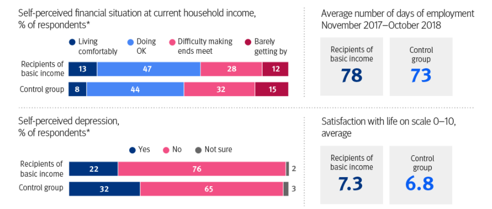
As Kela (2020) points out, although the employment increase was relatively small overall, for families with children who received a basic income, employment rates improved more significantly during both years of the experiment. In general, members of the treatment group were more satisfied with their lives and experienced less mental strain, depression, sadness, and loneliness. They also reported a more positive perception of their cognitive abilities (i.e. memory, learning, and ability to concentrate), and perceived their financial situations as being more manageable.

These results beg an important question when it comes to implementation of new and innovative PSE programs: In the absence of tangible results, such as changes in employment rates, are the intangible benefits experienced by participating Homo sapiens worth the social investment?

Microfinance

One of the more innovative approaches to financing small businesses in lower-income countries is known as microfinance (Banerjee, 2013; Mia et al., 2017). Bangladeshi social entrepreneur and 2006 Nobel Prize winner Mohammad Yunus is credited as being the progenitor of microfinance because of a project he initiated in 1976, providing small business loans to small groups of poor residents in rural Bangladeshi villages. The project subsequently led to the founding of Grameen Bank in 1983, whose guiding principle is that small, well-targeted loans are better at alleviating poverty than donor aid.

The basic idea behind microfinance is simple. Because traditional lending requirements in the banking industry rely on borrowers pledging significant collateral to protect the interests of the lender, and because the risk of the borrower defaulting on a bank loan is often large and potentially costly, bank loans are generally considered off-limits to poorer entrepreneurs. Microfinance solves this loan-inaccessibility problem by lending to groups of entrepreneurs who essentially form cooperatives to advance collective business interests and take collective responsibility for loan repayment. The pooling of risk within the group lowers the chance of default on a loan and helps ensure that the loan will be profitable for both the borrower and the lender—a classic “win-win” solution, at least for Homo economicus borrowers and lenders.

But what about Homo sapiens? Although evidence suggests that microfinance has typically been a win for Homo sapiens lenders in terms of high rates of loan repayment (and therefore, low default rates) (Banerjee, 2013; Mia et al., 2017), the proverbial jury is still out regarding the extent to which microfinance has been a win for Homo sapiens borrowers. In an extensive field experiment, Banerjee et al. (2015) surveyed a large sample of residents located in 50 randomly selected poor neighborhoods in Hyderabad, India where branches of the microfinance firm Spandana and, later, other firms, had recently been established.^[17] The authors surveyed the members of their sample three separate times—in 2005, 2007, and 2009 (i.e., before, during, and after the opening of the Spandana branches).^[18]

The authors found that borrowers used microfinance loans to purchase durable goods for their new or existing businesses that had hitherto been unaffordable without the loan money. The typical borrower repaid the loan by reducing consumption of everyday “temptation goods” and working longer hours. No evidence was found of the loans ultimately helping to lift borrowers out of poverty in terms of improved health, education, and empowerment. If the loans helped anyone, it was the relatively larger, already-established businesses with relatively high pre-existing profit levels. Less than 40% of eligible, or “likely borrowers” availed themselves of the microfinance loans even though they continued to borrow from other informal sources.

The evidence for micro-financed loans on the profitability of solely new businesses is likewise bleak. The authors find that new businesses between roughly the 35th and 65th percentiles of profitability have statistically significant lower profits in the neighborhoods where microfinance loans became available. Nevertheless, Banerjee et al. (2015) report that this overall result shields divergent effects across industry types. In particular, new food businesses (tea/coffee stands, food vendors, small grocery stores, and small agriculture) that availed themselves of micro-financed loans on average experienced an 8.5% bump in profitability relative to new food businesses that established themselves in neighborhoods without access to microfinance loans. In contrast, new rickshaw/driving businesses backed by microfinance loans experienced a 5.4% decline in profitability relative to new rickshaw/driving businesses that established themselves in neighborhoods without access to microfinance loans.

In conclusion, Banerjee et al. are balanced in their assessment of the findings. They conclude that microfinance is indeed associated with some business creation—in the first year after obtaining microfinance, more new businesses are created, particularly by women. However, these marginally profitable businesses are generally smaller and less profitable than the average business in the neighborhood. Microfinance also leads to greater investment in existing businesses and an improvement in the profitability of the most profitable among those businesses. For other businesses, profits do not increase, and, on average, microfinance does not help these businesses expand in any significant way. Even after three years of having assumed a microfinance loan, there is no increase in the number of these businesses’ employees (i.e., business size) relative to businesses that did not assume loans.

Once again, the fickleness of Homo sapiens plays itself out in a market setting, this time in the neighborhoods of Hyderabad, India.

Trust as Social Capital

In Section 2 we investigated the trust game and the extent to which Homo sapiens participating in laboratory experiments express both their trust and trustworthiness. Knack and Keefer (1997) seek to answer the question, do societies comprised of more trusting and trustworthy individuals, all else equal, perform better on a macroeconomic scale? What is the relationship between interpersonal trust and norms of civic cooperation (i.e., social capital) on the one hand, and economic performance on the other?^[19]

As the authors point out, conventional wisdom suggests that economic activities requiring agents to rely upon the future actions of others (e.g., transactions involving goods and services that are provided in exchange for future payment; employment contracts in which managers rely on employees to accomplish tasks that are difficult to monitor; or investments and savings decisions that rely on assurances by governmental agencies or banks that assets will not be appropriated) are accomplished at lower cost in higher-trust societies. Individuals in higher-trust societies spend less time and money protecting themselves from being exploited in economic transactions. Written contracts are less likely to be needed, and when needed, they are not required to specify every possible contingency. Litigation may be less frequent. Individuals in high-trust societies are also likely to divert fewer resources to protecting themselves from unlawful violations of their property rights (e.g., through bribes or private-security services and equipment). Further, high trust can encourage innovation. If entrepreneurs are required to devote less time to monitoring possible malfeasance committed by partners, employees, and suppliers, then they have more time to devote to innovation in new products or processes.

For their measures of trust and civic norms, Knack and Keefer utilize The World Values Survey, which contains survey data on thousands of respondents from roughly 30 different market economies worldwide. The survey question used to assess the level of trust in a society is this:

“Generally speaking, would you say that most people can be trusted, or that you can’t be too careful in dealing with people?”

Based upon survey participants’ responses, the authors created a trust indicator variable (TRUST) equal to the percentage of respondents in each nation replying that most people can be trusted. The extent of civic norms present in a given society is gleaned from responses to questions about whether each of the following behaviors can always be justified, never be justified, or something in between:

1. “claiming government benefits which you are not entitled to”
2. “avoiding paying a fare on public transport”
3. “cheating on taxes if you have the chance”
4. “keeping money that you have found”
5. “failing to report damage you’ve done accidentally to a parked vehicle”

Respondents chose a number from one (never justifiable) to 10 (always justifiable). The authors summed values over the five items to create a scale (CIVIC) with a 50-point maximum score. They then measured the impact of TRUST and CIVIC on both national growth (in terms of Gross Domestic Product (GDP)) and investment rates. To control for other determinants found in the literature on economic growth, Knack and Keefer included in their regression analysis the proportion of eligible students enrolled in secondary and primary schools in 1960 (positively related to growth), per capita GDP at the beginning of the study’s timeframe of analysis (negatively related to growth), and the price level of investment goods (also negatively related to growth).

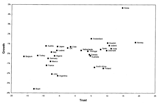
According to the figure below, which shows a scatter plot of the relationship between the countries’ TRUST and economic growth rates, the relationship appears to be positive (i.e., if you were to draw a line through the scattered points that represents a likely trend, the trend line would have a positive slope).

The table below presents the authors’ empirical results based upon different specifications for ordinary least squares (OLS) regression equations:

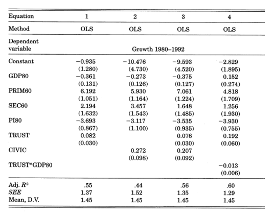
The social capital variables exhibit a strong and significant relationship to growth. For example, in Equation 1, the estimated coefficient for TRUST is positive (0.082) and statistically significant (due to its relatively low standard error of 0.030 in parenthesis). As Knack and Keefer explain, TRUST’s coefficient indicates that a ten-percentage-point increase in TRUST’s score is associated with an increase in economic growth of four-fifths of a percentage point. Similarly, according to CIVIC’s estimated coefficient, each four-point rise in the 50-point CIVIC scale in Equation 2 is associated with an increase in economic growth of more than one percentage point. When both social capital variables are entered together in Equation 3, their coefficient estimates drop slightly but remain statistically significant. Finally, the negative (and statistically significant) coefficient value on the interaction term TRUST*GDP80 indicates that the effect of TRUST on economic growth is lower for countries with higher initial per-capita GDP levels at the beginning of the timeframe of analysis, in 1980 (represented by variable GDP80).

Therefore, it seems that Knack and Keefer’s evidence of the extent to which trust and civic norms affect the welfare of a country supports the hypothesis that trust is indeed a form of social capital.

Reputational Effects

In Chapter 8, we learned of Fehr and Gächter’s (2000) finding that Reputational Effects among a group of repeatedly partnered players in a laboratory-conducted, finitely-repeated Public Good Game are capable of mitigating free-riding behavior among the players (i.e., contribution levels that are repeatedly too low to adequately fund the public good). Concern about one’s reputation among other players (for either strategic or non-strategic reasons) is a strong-enough incentive for players to voluntarily contribute at higher levels.

Curious about whether a Reputational Effect (or “indirect reciprocity”) is capable of promoting large-scale cooperation in real world settings, Yoeli et al. (2013) designed a field experiment involving over 2,400 customers of a California utility company, Pacific Gas and Electric Company, in order to study the customers’ levels of participation in a “demand-response program,” called SmartAC, designed to prevent electricity blackouts (before getting into the proverbial weeds of the experiment, convince yourself that participation in a prevention program like this indeed fits the definition of a public good).^[20] The authors’ hypothesis is that the effects of indirect reciprocity are strong in a setting such as this.

According to Yoeli et al., indirect reciprocity is based on repeated encounters in a group of individuals where my behavior toward you also depends on what you have done to others. We Homo sapiens have a relatively sophisticated social intelligence—we take a keen interest in who does what to whom and why. To be blunt, we gossip. And we are attuned to others’ gossip about us. Indirect reciprocity enables us to track the good and bad behavior of others and, when it comes to contributing toward a public good, to use this information to incentivize cooperation.

The authors informed customers about the program via mailers. Sign-up sheets were simultaneously posted in a communal area near their home, usually by a shared mailbox kiosk. Those who signed up to participate in the program allowed the utility to install a device that remotely curbed their central air conditioners when necessary—on days with unusually high demand or in the case of an unexpected plant or transmission failure. In their primary manipulation, Yoeli et al. varied whether residents’ neighbors could tell who had signed up for the program. They did so by dividing the publicly posted sheets between those requiring residents to print their name and unit number (observability treatment) and those providing a printed code number that did not reveal their identity (anonymous treatment). Note that participants in the observability treatment are susceptible to the effect of indirect reciprocity.

The figure below presents the experiment’s general result. We see that observability tripled participation in the program, suggesting that reputational effects are indeed present in this public good experiment. Note that because the “whiskers” (|) at the top of the two boxes do not overlap with each other, the difference between the participation rates is statistically significant.^[21]

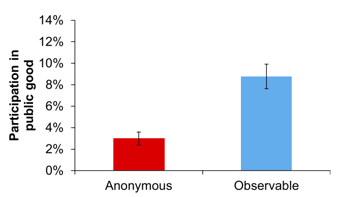
Charts A and B below dissect these results a bit further. In Chart A, we see that the observability treatment increased participation more in apartment buildings where residents are more likely to interact with their neighbors in public spaces, and sign-up sheets were posted in especially conspicuous locations, as compared with row houses or individual homes where neighbors are less likely to interact and sign-up sheets were less easily visible (note the lack of statistical significance for those living in homes—the whiskers overlap with each other). In Chart B, we see that the observability treatment increased participation more among those who own their homes/apartments relative to those who rent (note the lack of statistical significance for renters). The authors suggest that renters are more transient and therefore less likely to invest in long-term relationships with their neighbors.

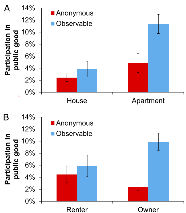
On a final note, Yoeli et al. provide evidence that indirect reciprocity among Homo sapiens is unique to public goods. Their hypothesis is that choosing not to participate in a demand response program should carry the threat of social sanctions only if participation is considered to be for the public good. To test their hypothesis, the authors solicited an additional 1,000 customers with exactly the same treatments as described above, except that the informational materials the customers received ahead of time to entice them to participate in the demand response program were stripped of any language that framed blackout prevention as a public good. In the figure below, we see that, relative to the first figure above, the effect of indirect reciprocity is dramatically reduced among participants who did not receive the public good framing.

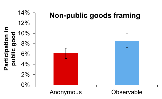
In the end, Yoeli et al.’s results suggest that Homo Sapiens are substantially more cooperative when their decisions are observable and when others can respond accordingly. The authors surmise that participants in their field experiment exhibited an understanding that having a good reputation is valuable in a public good setting and thus were willing to pay the cost of cooperation.

Employer-Provided Retirement Savings Plans

According to the Employee Benefits Research Institute (EBRI), less than a third of American workers feel very confident that they have saved enough money to live comfortably in retirement, and 60% report that preparing for retirement makes them feel stressed. Among those workers participating in an employer-sponsored, defined-contribution retirement plan, 80% report feeling satisfied with their plan and two-thirds are confident in their ability to choose the best-available retirement investments for their perceived situations. Only one-third were auto-enrolled into their plan. Overall, more than 30% of retirees feel that they do not have enough money saved to last their entire lifetimes (EBRI, 2020).

It is commonly believed that workers who fail to join an employer-sponsored plan, or who participate in the plan at low levels, appear to be saving less than they should for retirement—a mistake Homo economicus would naturally avoid making. In explaining this suboptimal behavior among Homo sapiens, behavioral economists stress lack of self-control, which leads to time-inconsistent investment choices being made over the course of a worker’s career due to procrastination or Status Quo Bias. One potential solution to this problem has been for employers to automatically enroll their employees into a default plan, which then requires the employee to “opt-out” if they wish to make any changes to the default savings portfolio at any time during their employment.^[22] The question of how workers should adjust their savings rates and portfolio allocations over time to ensure they are saving appropriately to meet their expected retirement needs looms large.

To overcome this potential time-inconsistency problem, Thaler and Benartzi (2004) proposed a new retirement savings program called Save More Tomorrow (SMarT). The program’s commitment mechanism is straightforward. People commit now (when they begin the program) to increase their savings rate later (each time they get a pay raise). In other words, workers could continue to procrastinate about saving more for retirement over time and, in the end, still save more. Beautiful!

Thaler and Benartzi implemented the SMarT program as a natural experiment at an anonymous, mid-sized manufacturing company. The authors found that roughly 80% of those workers who were offered the plan joined, and 80% of those who joined it remained in the plan through a targeted fourth pay raise. The average saving rates for SMarT program participants increased from 3.5% to 13.6% over the course of a monitored 40 months. Employees who accepted an alternative saving recommendation increased their saving rate to a lesser extent, and those who declined both the SMarT and alternative savings plans saw no increase in their savings rate over the 40-month period.

Thaler and Benartzi find that more than half (162 out of 315) of the company’s employees given the opportunity to participate in the SMarT program chose to do so. At the time of their first pay raise, the average savings rate for SMarT participants was equal to the average for those employees who made no effort to even contact the company’s financial consultant, but less than the average savings rate for those who did contact the consultant and chose to adopt the consultant’s recommended rate of slightly over 9%. However, by the second pay raise, SMarT participants were saving at a higher rate than any other employee group, and the differential in rates increased over the course of the subsequent two pay raises. It seems the SMarT program was successful in overcoming the employees’ time-inconsistency problem with respect to biting the proverbial bullet and saving for retirement. SMarT was indeed a smart way to nudge workers into saving more for their retirements.

Public Retirement Savings Plans

In contrast to private retirement savings plans like SMarT, Thaler and Sunstein (2009) describe Sweden’s launch of an innovative public retirement savings program in 2000 aimed at overcoming potential time-inconsistent behavior among the country’s workforce. All workers were instructed to choose between a default (opt-out) program designed by the national government or their own customized (opt-in) investment portfolio. By 2006, only 8% of new enrollees were customizing their own portfolios. This suggests that a sizable percentage of Swedish workers either recognized their penchant—as Homo sapiens—for making sub-optimal time-inconsistent decisions when it comes to saving for retirement, or they simply procrastinated their way into the default program.

On average, individuals who chose their own customized portfolio invested more in equities (particularly in Swedish equities) than those choosing the default program. The default portfolio was more diversified, more heavily invested in index funds, and carried a lower fee. Most importantly from the investor’s perspective, the default portfolio earned less-negative returns during the first three years and markedly higher positive returns over the subsequent three-year period.

Skål (as they are fond of saying in Sweden) to all the default Swedish savers! They responded well to the nudge of saving more for retirement.^[23]

The Deadweight Loss of Gift-Giving

Ho Ho Ho, or Ha Ha Ha? That’s the question Waldfogel (1993) set out to answer about the time-honored tradition of gift-giving (e.g., during Christmas, Hanukkah, Valentine’s Day, Mother’s Day, weddings, births, etc.). Is the spirit of gift-giving (Ho Ho Ho) strong enough on its own merits to outweigh the potential deadweight loss imposed on Homo sapiens gift-givers and gift-recipients as a result of the gifts given (Ha Ha Ha)? As Waldfogel points out, an important feature of gift-giving is that consumption choices are made by someone other than the final consumer. As a result, gifts may be mismatched with the recipients’ preferences. According to the rational model of choice behavior, the best a Homo economicus gift-giver can do with, say, $10, is to duplicate the choice that the recipient would have made. Because he implicitly solves the problem of maximizing the recipient’s utility, a Homo economicus gift-giver gives cash if his perception of the recipient’s utility from the cash gift, say $10, exceeds his perception of the recipient’s utility from a non-cash gift costing $10.

While it is possible for a gift-giver to choose a non-cash gift that the recipient ultimately values above the price paid by the giver (e.g., when the recipient is not perfectly informed about a gift that she really enjoys), when it comes to Homo sapiens gift-givers, it is more likely the gift will leave the recipient worse off than if he had made his own consumption choice with an equal amount of cash. In short, gift-giving among Homo sapiens is a potential source of deadweight loss (terminology economists use to denote inefficiency) when the costs of something (in this case, gifts paid for by gift-givers) outweigh its associated benefits (recipients’ valuations of their gifts plus the value gift-givers derive from the act of gift-giving itself).

Waldfogel estimates the deadweight loss of holiday gift-giving based upon surveys given to a group of Yale undergraduate students. He ultimately finds that holiday gift-giving results in deadweight loss ranging from 10% to a third of the value of gifts given. Non-cash gifts from friends and significant others are found to result in the least amount of deadweight loss, while those from members of the extended family result in the most. Given that holiday expenditures in the US in the 1990s averaged $40 billion per year, this would suggest a deadweight loss ranging from $4 billion to over $13 billion per year.^[24]

Waldfogel’s field experiment consisted of a series of two surveys administered to roughly 100 students over the course of three months. In the first survey (completed after the Christmas season in January of 1993), the students were asked to estimate the total amounts paid by their respective gift-givers for all of the holiday gifts they received the previous month. Students were asked to place a value on each of their gifts based upon their hypothetical willingness to pay (WTP) for each gift and whether they later chose to exchange any of their gifts. The second survey (completed in March 1993) gathered additional data on each respondent’s individual gifts listed in the first survey. The second survey asked respondents to describe each of their gifts, identify the givers’ ages and relationships to the recipient (i.e., parent, aunt or uncle, sibling, grandparent, friend, or significant other), estimate the prices that the givers paid for the gifts, and indicate whether the gifts were ultimately exchanged. The gift description allowed the gifts to be divided into three categories: cash, gift certificates, and non-cash gifts. Perhaps most importantly, the students were again asked to place a value on each of their gifts, but this time based upon their hypothetical willingness to accept (WTA) payment for giving the gifts up.

In Survey 1, Waldfogel finds that students estimate that friends and family paid an average of roughly $438 for the recipients’ total gifts, but the students express an average WTP (or value) of only $313 for the same gifts. The ratio of average WTP to average price paid (71.5%) suggests an average deadweight loss of roughly one-third of the value of all gifts given. Results from Survey 2—based upon the students’ WTA values rather than WTP—suggest a deadweight loss closer to 10% of the value of all gifts given. Recall from Chapter 5, Homo economicus and the Endowment Effect, that we generally expect WTA values to exceed WTP values, which could explain Survey 2’s lower estimates of deadweight loss from gift-giving.

Waldfogel goes on to report that aunt/uncle and grandparent gifts were the most likely to be exchanged, at rates of just under 21% and just over 13%, respectively. Ten percent of non-cash gifts received from parents were exchanged, as were roughly 7% of gifts from siblings and friends. A negligible number of gifts received from significant others were exchanged. Deadweight losses are larger for gifts given by extended family than by the immediate family, and losses increase with the age difference between the giver and recipient.

Recall that Waldfogel’s deadweight-loss estimates were based upon hypothetical WTP and WTA values elicited from two survey instruments. List and Shogren (1998) put Waldfogel’s findings to the test by instead eliciting valuations of an individual’s gifts using an actual (i.e., real) “random nth price auction” in an effort to reduce potential Hypothetical Bias associated with Waldfogel’s WTP and WTA estimates. As List and Shogren describe it, the auction works as follows:

1. For each gift received, an individual states his total value to sell the gift (i.e., states his WTA).
2. All gifts for a given individual, , where equals both the given individual’s last gift and his total number of gifts, are then pooled together to create the set of total gifts across all individuals, , where represents the total number of individuals participating in the experiment.
3. The set of total gifts, , is then rank-ordered from lowest to highest gift number across the individuals.
4. The experimenter then selects a random number, , uniformly distributed between 2 and 21 (2 was the lowest and 21 the highest number of gifts received by the individuals participating in the experiment).
5. The experimenter then purchases (with real money) the () lowest total value (i.e., lowest WTA) gifts overall and pays the th lowest total value for each gift. For example, suppose = 6. Then, only the five lowest-valuation gifts overall (across the individuals) would be purchased at the sixth lowest WTA value.

Complicated? A bit. But it seems a small price to pay (no pun intended) to mitigate potential hypothetical bias. List and Shogren go on to estimate a welfare gain associated with gift-giving—their average percentage yields range between 121% and 135% (as opposed to Waldfogel’s 66% and 87% from the table above). Hence, it appears that evidence concerning gift-giving is context-specific—it depends upon how a given experiment is designed or framed. Hypothetical surveys suggest the existence of a deadweight loss. Real auctions suggest the existence of welfare gains. It seems we’ve been framed again by Homo sapiens.

The Behavioral and Psychological Effects of Money

As Heyman and Ariely (2004) point out, Homo sapiens often solicit help with tasks such as moving their possessions to a new residence, painting a room, or taking care of their kids. When we ask for help, we may wonder whom to approach and how best to motivate him or her. Should we ask a professional or a friend? If we ask a friend, should we offer compensation? If so, how much should we offer, and what form of compensation would be most effective? Would cash or personal gifts provide a stronger incentive? Using monetary payments causes participants to invoke monetary-market frames and norms. When money is not involved (i.e., there is either payment in the form of a gift or no payment is made at all), the market is perceived to be a social market invoking social norms. The authors discuss a set of experiments they designed to demonstrate that monetary vs. gift payments have material consequences for the payment-effort trade-off. Note that there is no such trade-off in the mind of Homo economicus. Homo economicus simply calculates the monetary value of the gift payment and thereby obviates any inherent distinction between the cash- and gift-payments.

In one experiment (Experiment 2), approximately 160 students each repeatedly dragged a computerized ball to a specified location on a computer screen. The software explained to the participants that a light gray circle (the ‘‘ball’’) would appear on the left-hand side of the screen and that their task was to drag as many of these balls as they could into a dark gray square on the right-hand side of the screen over the course of a three-minute period. Next, participants saw a screen that informed them of the payment they would receive (unless they had been randomly selected into the control condition of no payment). Those randomly assigned to the cash-payment treatment were paid in cash and those assigned to the gift-payment treatment were paid in an equivalent amount of Jelly Belly jellybeans.

Participants were not told the market price of the candy. The level of payment was either low (10 cents in the cash-payment treatment or five Jelly Bellies in the gift-payment) or medium ($4.00 in the cash-payment treatment or a half pound of Jelly Bellies in the gift-payment treatment). Results from this experiment are depicted in the figure below.

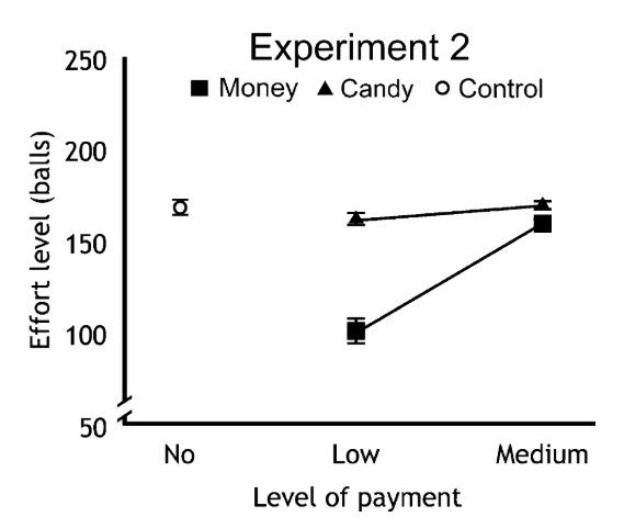
We see four key results in this figure. First, the average participant’s effort level (with respect to the ball-dragging task) in the cash-payment treatment increased significantly when the payment level increased from low to medium. Second, effort level in the gift-payment treatment is insensitive to the increase in payment level from low to medium. Third, effort level in the low-payment level of the cash-payment treatment is significantly below that of the no-payment control condition, but effort in the low-payment level of the gift-payment treatment is not. Lastly, the difference in the effort levels in response to the low level of payment in both the cash- and gift-payment treatments is statistically significant. In summary, these results support the distinction between monetary and social markets. In particular, they demonstrate that the decrease in performance from no-payment to low-payment conditions is found in monetary exchanges, but not in gift exchanges.

In another experiment, Heyman and Ariely tested the effects of monetizing the value of the gift payment (e.g., rather than valuing the low-payment gift as five Jelly Bellies, it was described as 10 cents worth of Jelly Bellies). The authors’ prediction was that once the retail value of the candy was mentioned, the average participant’s effort would be similar to that observed in the cash-payment treatment (i.e., the Homo sapiens participants would have no reason not to behave like Homo economicus). This is indeed what occurred, leading Ariely (2008) to state that “Once the bloom is off the rose—once a social norm is trumped by a market norm—it will rarely return” (page 85).

Ariely (2008) eloquently extrapolates the results of these experiments to a broader social context:

“If corporations started thinking in terms of social [markets], they would realize that these [markets] build loyalty and—more important—make people want to extend themselves to the degree that corporations need today: to be flexible, concerned, and willing to pitch in. That’s what a social relationship delivers.” (page 90)

Hence, in the less-predictable world of Homo sapiens, businesses must decide the extent to which they participate with their employees and customers in monetary and/or social markets.

As a follow-on to Heyman and Ariely’s (2004) experiments exploring the payment-effort trade-off, Vohs et al. (2006) sought to understand the behavioral psychology underscoring the trade-off. In its most general terms, the authors’ hypothesis is that money makes Homo sapiens feel self-sufficient and behave accordingly. When reminded of money, people desire to be free from dependency upon others and prefer that others not depend upon them. Vohs et al. designed several experiments to test this hypothesis from a variety of angles.

In one experiment, the authors found that participants (a sample of University of Minnesota students) who were reminded about money—both Monopoly money and real money—in the context of a series of word descrambling tasks worked longer at the tasks than participants in a non-money-primed control group before requesting help from the experimenter.^[25] In subsequent experiments with different groups of students, Vohs et al. found that (1) participants in a high-money treatment worked significantly longer than participants in a low-money treatment before asking for help from another available participant, (2) participants in a money-primed treatment volunteered to help code fewer data sheets than did participants in the non-money-primed control condition, (3) participants in a high-money treatment volunteered to gather fewer pencils that had spilled onto the floor than did participants in a low-money treatment, and (4) participants in a money-primed treatment donated significantly less money to a university student fund than participants in the non-money primed control. Three final experiments tested the effects of money on social intimacy, desire to engage in leisure activities alone, and preference to work alone. As expected, participants who were primed with money ahead of time were subsequently less socially intimate and exhibited a stronger preference for engaging in leisure activities and working alone.

So yes, Vohs et al.’s experiments suggest that money makes Homo sapiens feel self-sufficient and behave accordingly.

Price and The Placebo Effect

Is it possible that the magnitudes of placebo effects experienced by Homo sapiens (e.g., through medical therapies or medications) are somehow influenced by the prices we pay for them? To investigate this possibility, Waber et al. (2008) studied the effect of price on a group of Homo sapiens’ analgesic responses to placebo pills. Over 80 healthy volunteers in Boston, MA were recruited via an online advertisement to participate in a field experiment where each participant was informed by a brochure about a purported new opioid analgesic recently approved by the Food and Drug Administration. The opioid was described as similar to codeine but with a faster onset time. In reality, and not disclosed to the participants, the pill was a placebo. After randomization, half of the participants were informed that the drug had a regular price of $2.50 per pill (“regular price”), and half of the participants that the price had been discounted to $0.10 per pill with no reason mentioned for the price discount (“low price”).

The experiment followed the established approach for studying electrical shocks which were administered to the wrist and calibrated to each participant’s pain tolerance level. After calibration, participants received the test shocks, rating the pain on a computerized visual analog scale anchored by the labels “no pain at all” and “the worst pain imaginable.” Participants received shocks in 2.5-volt increments between 0 volts and their calibrated tolerances. Shocks at each intensity level were carried out twice for each participant (before and after taking the pill), and the change in reaction to the shock was assessed.

The authors found that, when informed of the regular price, slightly over 85% of the participants experienced pain reduction after taking the pill. This was a significantly higher percentage than the slightly over 60% of participants who reported pain reduction when informed of the low price. Waber et al. also found that for 26 of 29 intensities (from 10 to 80 V), average pain reduction was assessed as being greater for the regular-priced than the low-priced pill. Those informed of the regular price reported experiencing greater pain reduction beginning at roughly 25 volts (the authors report that the mean differences are statistically different for the shock intensities of 27.5 volts through 30 volts, 35 volts through 75 volts, and at 80 volts). In other words, Waber et al. found an abundance of evidence suggesting that Homo sapiens do indeed correlate perceived reductions in pain (as induced by placebo effects) with the placebo’s per-unit price. Placebo effects are perceived to be more effective as they become more expensive. Ouch.

The Effects of Conceptual Information on the Consumption Experience

To what extent does conceptual (e.g., imaginary) information about a good and a consumer’s expectations about the quality of that good influence the consumer’s subjective experience of consuming the good? As early experiments with consumers demonstrated, Homo sapiens’ preferences can indeed be influenced by conceptual information. For example, McClure et al. (2004) found in their experiments that Coca-Cola was rated higher when consumed from a cup bearing the Coca-Cola brand logo rather than from an unmarked cup. Wansink et al. (2000) similarly found that describing the protein of nutrition bars as ‘soy protein’ caused them to be rated as more-grainy and less-flavorful than when the word ‘‘soy’’ was removed from the description. However, as Lee et al. (2006) point out, none of these early experiments measured the extent to which information disclosure affected the consumption experience itself (i.e., the perceived tactile quality of the good). The experiments instead merely measured the consumer’s retrospective interpretation of the experience.

To better answer the question of how conceptual information affects the consumption experience, Lee et al. conducted a series of field experiments. In each experiment, participants consumed two beer samples: one unadulterated sample and one sample of ‘‘MIT brew” containing several drops of balsamic vinegar, a beer flavoring that most participants found conceptually offensive. Participants were randomly assigned to one of three treatments. In the “blind treatment,” the participants tasted the two beers without any information provided about the contents, and then indicated their preferences. In the “before treatment” they were told which beer contained balsamic vinegar prior to tasting it, after which they indicated their preferences. In the “after” treatment the respondents tasted the beers, were then told which of the beers contained vinegar, and then indicated their preferences. Note that because the information about the MIT brew concerns something considered conceptually offensive, the information itself is, by default, conceptual.

The authors point out that if the balsamic vinegar’s presence solely affects preferences, the timing of the information should not matter, and preferences for the MIT brew should be reduced equally in the before and after treatments relative to the blind treatment (i.e., blind > before after). In contrast, if the information influences the consumption experience itself, preference for the MIT brew should be markedly lower in the before treatment than in the after treatment (i.e., blind after > before).

The experiments were conducted at two local pubs: The Muddy Charles and The Thirsty Ear. A total of approximately 400 patrons of these two pubs tasted two 2-oz. samples of beer each. One sample was of unadulterated beer (Budweiser or Samuel Adams) and the other of MIT brew. Participants in Experiment 1 merely indicated which of the two samples they liked best. In Experiment 2, participants also received a full (10-oz.) serving of the sample they preferred. In Experiment 3, the blind treatment was the same as in Experiment 2, but in the before and after treatments, participants received a full (10-oz.) glass of regular beer, some balsamic vinegar, a dropper, and the ‘‘secret recipe’’ (‘‘add three drops of balsamic vinegar per ounce and stir’’). The figure below depicts Lee et al.’s results:

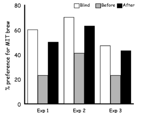
We see that in each experiment preference for MIT brew is (1) significantly higher in the blind treatment than in the before treatment, (2) significantly lower in the before treatment than in the after treatment, and (3) not significantly different across the blind and after treatments. In other words, blind after > before. Thus, the authors indeed find evidence that conceptual information—in this case, about something considered conceptually offensive—influences the consumption experience itself. Conceptual information can indeed alter Homo sapiens’ expectations about the goods they consume.

Can Default Options Save Lives?

Johnson and Goldstein (2003) were motivated to ask this question because of glaring differences persisting between the US and several European Union nations when it comes to the role organ donations play in the saving of lives. In the US, thousands of patients die each year waiting for organ donations in spite of an oft-cited Gallup poll showing that (1) 85% of Americans approve of organ donation, (2) less than half of the American adult population have made a decision about donating, and (3) less than 30% have granted permission to harvest their organs by signing a donor card (Gallup, 1993). In the US, organ donation must be opted into via explicit consent, as it is in the United Kingdom, Germany, the Netherlands, and Denmark. To the contrary, in other European Union nations (e.g., Austria, Belgium, and France), organ donation must be opted out of. As Johnson and Goldstein show in the figure below, among European countries, the difference in effective consent percentages (ECPs) between explicit- and presumed-consent is stark:

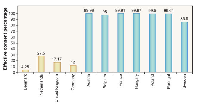
The ECP is the percentage of citizens who have opted in to donate their organs in explicit-consent countries, and the percentage who have not opted out in presumed-consent countries. In the figure, countries whose ECPs are represented by the gold bars are explicit-consent, and the countries whose ECPs are represented by the blue bars are presumed-consent. A picture is worth a thousand words here. On average, 60 percentage points separate the two groups.

To explain this difference, Johnson and Goldstein propose three possible reasons. First, citizens might believe that defaults are suggestions by their country’s policymakers that imply a recommended action. In explicit-consent countries, the suggestion is to think hard about opting in, while in countries with presumed-consent the suggestion is to think hard about opting out. Second, since making a decision often entails effort and stress, whereas accepting the default is effortless, many people choose to avoid making an active decision about donating their organs. Third, default options often represent the status quo, and thus, change entails a trade-off. Due to loss aversion (which, as we know, is common among Homo sapiens), perceived losses associated with changing one’s organ-donation status loom larger than equivalent gains.

The authors further investigate the effect of default options on donation rates by conducting an online experiment with over 160 respondents. The respondents were asked whether they would choose to become donors based upon one of three questions pertaining to different default options. In the question worded for the opt-in option, participants were told to assume that they had just moved to a new state where the default option was to not become an organ donor, and they were asked to confirm or change that status. The question for the opt-out option was worded identically, except that the default option was to become a donor. The third question was worded for a neutral condition, which simply required a respondent to choose whether to become a donor without any particular default option. Resulting ECPs are depicted in the figure below:

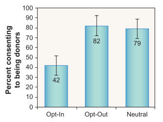
As the figure shows, the specific wording of the question had a dramatic impact. Stated ECPs were about twice as high when the respondent had to opt-out rather than opt-in. The ECP associated with the opt-out option did not differ significantly from the ECP for the neutral condition (without a specified default option provided). Only the ECP associated with the opt-in option, which represents the current practice in the US, was significantly lower than the ECP for the opt-out option.

The moral of this story, like that of the private and public retirement-savings stories encountered previously, is that merely framing a socially desirable choice as an opt-out decision can nudge Homo sapiens in the socially desirable direction.

Reward Versus Punishment

Although not the domain of behavioral economists per se, the question of rewarding good behavior versus punishing bad behavior is a perennial one for anyone tasked with having to manage another’s behavior or choices that determine a shared outcome—think parent-child, manager-worker, policymaker-citizen relationships. Do rewards for improved performance motivate better (i.e., nudge more) than punishments for mistakes?

Neuroscientists would argue that it depends. For example, Wachter et al. (2009) argue that rewards enhance learning in Homo sapiens, whereas punishment tends to improve motor performance. As Fryer et al. (2012) showed previously, rewards can work, particularly when framed as losses. Recall that the authors showed that teachers in Chicago (of K-8 students) who were paid in advance and asked to give the money back if their students did not improve sufficiently improved their students’ math test scores. Teachers who were paid traditional subsidies for improved student performance did not improve their students’ scores. And when it comes to reducing crime through greater punishment—in particular, higher arrest rates—Levitt (1998) showed that greater punishment can reduce certain types of crime, but not necessarily all types.

In one of the most highly cited field experiments involving the use of punishment, Gneezy and Rustichini (2000) found that punishment, if not administered at the correct level, can backfire, leading to more (not less) of the undesirable behavior. In their study of parents who were habitually late in picking up their children at Israeli daycare centers, a new fine levied on parent tardiness actually exacerbated the problem and ultimately led to adaptive behavior on the part of tardy parents. The authors concluded that penalties which are usually introduced into an incomplete social or private contract may change the information and perception among those being penalized regarding the environment in which they operate. The deterrence effect on behavior may therefore be opposite of what was expected.

Gneezy and Rustichini conducted their experiment at 10 daycare centers over a period of 20 weeks. In the first 4 weeks, they simply observed the number of parents who arrived late. At the beginning of the fifth week, they introduced a fine at six of the 10 daycare centers. The fine was imposed on treatment groups of parents who arrived more than 10 minutes late. No fine was introduced at the four other daycare centers, which served as the study’s control groups. After the introduction of the fine, Gneezy and Rustichini observed a steady increase in the number of parents coming late. At the end of an adjustment period that lasted 2–3 weeks, the number of late-coming parents remained stable at a rate higher than during the no-fine period. The fine was removed (without explanation to the parents) at the beginning of the seventeenth week. In the following four weeks, the number of parents coming late remained at the same high level as the previous period, which was higher than during the initial four weeks. In other words, on average tardiness actually increased and was sustained among tardy parents with the onset of the fine, even after the fine was eventually eliminated.

One explanation for this perverse deterrence effect is simply that the fine was set too low. It could very well be that $3 per child was interpreted by some parents as signaling that tardiness was not considered by their daycare center to be a major problem. Paying what they consider to be a relatively low fine actually served to sanction their tardiness by relieving the guilt they otherwise might have felt in habitually arriving late to pick up their child. In this sense, the parents’ willingness-to-pay (WTP) to relieve their guilt was greater than $3 per child. They were getting a deal!

Setting a fine or tax at the appropriate (or what economists call the “socially efficient”) level is generally considered to be an antidote. For a recent example, Homonoff (2018) found that taxes (punishment) reduce demand for plastic grocery bags, whereas subsidies (reward) on reusable bags do not. Likewise, Haselhuhn (2012) found that a large fine boosts compliance more than a small fine, but the influence of paying both large and small fines decays sharply over time. This latter finding suggests that while Homo sapiens can react rationally to these types of nudges, their reference points die hard (or, should I say, evolve stubbornly over time). Because their effects can be transitory, penalties and rewards seen as being temporary are unlikely to establish a “new normal” that policymakers may be striving for.

Indeed, a growing body of research suggests that in certain circumstances, both penalties and rewards can backfire by crowding out Homo sapiens’ intrinsic motivations and commitments to improve their behaviors, simply because the penalties and rewards are extrinsic (i.e., monetary) rather than intrinsic. For example, in their study of farmers in the La Sepultura Biosphere Reserve in Chiapas, Mexico, García-Amado et al. (2013) found that the more years a farmer has participated in a scheme where he is monetarily compensated for refraining from cutting down trees, hunting, poaching, or expanding the household’s cattle herds, the more the farmer’s stated preference for conserving the forest becomes financially driven. Further, a farmer’s readiness to participate in future conservation efforts increasingly depends upon promised future payments. To the contrary, in other parts of Chiapas where the forest is communally managed, more time is initially required to galvanize farmer engagement, but their motivation remains centered on the intrinsic benefits of long-term forest conservation.

Beware the longer-term impacts of monetary incentives!

Contingency Management of Substance Abuse

According to GBD 2016 DALYs and HALE Collaborators (2017), drug-use disorders are the 15th leading cause of disability-adjusted life years in high-income countries. Cocaine and amphetamines are the most commonly abused stimulants in people aged 15–64 years, with an annual prevalence of misuse among the global population of 0.38% and 1.20%, respectively (United Nations Office on Drugs and Crime, 2017). On the surface, these percentages may seem low, yet as the indirect effects on family members, friends, co-workers, and society at large of substance-abuse behavior are accounted for, virtually no one is unaffected.

As Degenhardt and Hall (2012) point out, patients addicted to stimulants experience a range of psychological and physical problems, including psychosis and other mental illnesses, neurological disorders, cognitive deficits, cardiovascular dysfunctions, sexually transmitted diseases, and blood-borne viral infections such as HIV and hepatitis B and C. Traditional approaches to recovery and rehabilitation, known as structured psychosocial interventions, tend to be expensive, embarrassing, difficult to access, and often ineffective (DynamiCare Health, 2020). These approaches eschew the use of explicit rewards and punishments, which, as we have previously learned, can be effective in altering a wide range of behaviors. So, why wouldn’t reward schemes work against substance use disorders (SUDs) (e.g., in response to a patient maintaining drug-free urine samples over a specified period of time)?

As it turns out, clinical experiments with SUD reward schemes, commonly known as Contingency Management (CM), have a relatively long history, particularly in the short- and long-term treatment of people with cocaine and/or amphetamine addiction. Based upon their meta-analysis of 50 independent randomized control trials, De Crescenzo et al. (2018) conclude that CM, particularly in combination with community reinforcements (i.e., interventions involving functional analysis, coping-skills training, and social, familial, recreational, and vocational reinforcements), is the only intervention among traditional 12-step programs, Cognitive Behavioral Therapy (CBT), motivational interviewing, and non-contingent reward programs that increase the number of abstinent patients at the end of treatment (short-term), again at 12 weeks (medium term), and later still (longer-term).

Vincz (2020) reviews an ongoing telehealth recovery program undertaken by Horizon Blue Cross Blue Shield of New Jersey and DynamiCare Health involving approximately 300 patients struggling with SUD. Participants are required to pay a non-refundable $50 participation fee (which can be earned back within the first month through the program’s reward system). They are then matched with a recovery coach (who are in recovery themselves) and receive breath and saliva testing equipment that works via a mobile app to support recovery remotely. The breath and saliva tests are conducted remotely through the app, relying on selfie video for verification. For staying sober and staying in treatment, members can earn monetary rewards worth up to $500 over the course of the 12-month program. The rewards come loaded on a smart-debit card which blocks access to bars, liquor stores, and cash withdrawals in order to protect the patient from risky spending.

The mobile app uses GPS technology to automatically check members into everything from medical appointments to Alcoholic Anonymous meetings, and record and reward patients for their participation in telehealth meetings and appointments. The app also contains a library of self-guided therapy modules based upon CBT. The short lessons teach crucial recovery skills such as how to deal with cravings, triggers, loneliness, and boredom.

If anything, this telehealth recovery program serves as an example of how a reward scheme paired with modern technology can be applied to one of society’s most pernicious and persistent problems, and, to some extent, nudge us toward making healthier choices.^[26]

F#!*ing Pain Management

Cognitive scientists posit several reasons and motivations for why Homo sapiens swear. Swearing is an efficient way to convey emotion, it is cathartic, and it is an inexorable part of human evolution accompanying our innate fight-or-flight reactions (Bergen, 2016). But as Bergen and others point out, swearing can also serve as a mental analgesic, helping us cope with both physical pain and pain associated with social outcomes, such as ostracism.

Stephens and Robertson (2020) set out to test this assertion by generating two non-pre-existing “swear” words—“fouch” and “twizpipe”—that could conceivably be used in place of a conventional swear word—you guessed it, “fuck”—and to assess the pain-relieving effects associated with repeating these words in the context of an ice-water pain challenge.^[27] A neutral word describing a standard wooden table (e.g., “solid”) was used as a control condition to provide a reference against which to assess the effects of the conventional and new swear words. The authors hypothesized, inter alia, that the average Homo sapiens’ pain threshold and tolerance levels would be higher for “fuck,” “fouch,” and “twizpipe” vs. the neutral word.

Approximately 100 students from Keele University participated in multiple trials of the experiment. For each student, the instructions for the ice water immersion were as follows:

In a moment, I would like you to fully immerse your nonpreferred hand into this ice water bath. While it is submerged, please repeat the word [INSERT AS APPROPRIATE] at normal speech volume and a steady pace, once every 3 seconds. While you have your hand in the water, I would like you to do TWO more things. First, please tell me when it becomes painful but don’t take your hand out yet unless you have to. Second, please try and keep your hand in the water for longer, taking it out when the pain becomes unbearable.

Timing began when the student’s hand was fully immersed and stopped when her hand was fully removed from the water. Immediately after each submersion, participants immersed their hand in a room-temperature bath for three minutes prior to the next ice-bath submersion. Stephens and Robertson find that utterance of the swear word “fuck” not only induces significantly higher pain threshold and tolerance levels than the neutral word (measured by the number of seconds that the average participant’s hand is submersed in the ice bath), but also higher levels of pain threshold and tolerance than the made-up swear words “fouch” and “twizpipe”. The authors find no statistical difference between the effects on pain threshold and tolerance of uttering “fouch” and “twizpipe” relative to the neutral word.

This suggests that when Homo sapiens decide to manage their pain with repeated utterances of a swear word, not just any word will do. Like the practiced eye of any connoisseur, the average Homo sapiens’ ear can distinguish authentic from spurious swear words. It is unclear whether Homo economicus’ ear is capable of such discernment.

Willingness to Accept Pain (WTAP)

Yes, you’ve read that correctly—WTAP, or Willingness to Accept Pain. We’re not talking about WTP (i.e., willingness to pay from Chapter 6 (recall Homo economicus and the Endowment Effect)). WTAP and WTP are two different things. For starters, while WTP is measured in dollars, WTAP is denominated in minutes (of pain tolerated). As such, WTAP is more similar to WTA (i.e., willingness to accept) than WTP. WTAP measures an individual’s willingness to accept an additional dose of painful experience in exchange for a given monetary payment.^[28] In Read and Loewenstein’s (1999) field experiment, WTAP is defined specifically as the amount of time a subject is willing to keep her hand submerged in the ice water for $1, $3, and $5.

Read and Loewenstein subjected their experiment’s participants (roughly 80 students and staff at the University of Illinois, Urbana-Champaign) to a 30-second ice-water pain challenge with the goal of measuring their WTAP with respect to their memories of the pain. Subjects either attended to the sensations of cold (sensation-focus condition, henceforth denoted as SENS) or were led to believe that the experiment was about manual dexterity (distraction, henceforth DIS). Subjects randomly assigned to the SENS condition were informed that the study was designed to assess the perception and memory of cold, while those assigned to the DIS condition were informed that the study was designed to assess manual dexterity under conditions of cold. In both conditions, subjects held a nut and bolt in their submerged hand and screwed and unscrewed the nut with their thumb and forefinger. Subjects in the DIS condition were told that their performance on this task was the focus of the study, while those in the SENS condition were not. WTAP was measured either immediately after pain induction (IMM) or following a delay of one week (DEL). Thus, there were four distinct experimental conditions: SENS/IMM, DIS/IMM, SENS/DEL, and DIS/DEL.

Read and Loewenstein’s experiment spanned three consecutive weeks. In week 1, all subjects except those in a control group underwent pain induction. They grasped a large metal nut and bolt in their right hand and then immersed this hand into an insulated, two-liter bucket filled with ice water for 30 seconds. While their hand was immersed in the water, they undid the nut from the bolt and then tightened it back on using their thumb and forefinger, repeating the task until the experimenter instructed them to stop. Following pain induction, the delay groups were scheduled to return in a week and then dismissed.

At this point (in Week 1 for the subjects in the IMM and control conditions, but in Week 2 for the subjects in the DEL condition), all subjects stated their WTAP for the first time (WTAP1). They were presented with the three money amounts ($1, $3, and $5) along with five time intervals for subsequent submersions of their hand in the cold bath (1, 3, 5, 7, and 9 minutes). Each of the 15 money-and-time combinations was written on a separate line, and subjects ticked off a box corresponding to “yes” (indicating that they were willing to immerse their hand in ice-cold water for that time in exchange for money) or “no” (indicating that they were not). Subjects were told that when they returned one week later, one of the money and time combinations would be chosen randomly and that their decision for that combination would “count.” This meant that if they checked “yes” for a combination and that combination was randomly chosen in the draw, then they would be instructed to immerse their hand in the ice water for the specified period and would be paid the agreed upon amount for doing so. If they failed to hold their hand in the water long enough, they would not receive the extra money. If they had checked “no” on the chosen line, they would neither be asked to submerge their hand nor receive any extra payment. Although they were later given a chance to change their minds (WTAP2), at the moment when they made their first choices, subjects were led to believe that these choices would count.

The authors hypothesize that average WTAP1 estimates would be ordered in the following way (note that for WTAP1, smaller numbers mean that pain is judged to be greater):

.

In other words, Homo sapiens judge pain assessed immediately after its occurrence to be greater than pain assessed after a delay of one week, all else equal. Among those assessing the pain immediately, those whose minds were distracted during the painful experience assess the pain to be greater than the pain suffered by those who were allowed to focus on the sensation of pain. Among those assessing the pain with a time delay, this relative assessment of the pain was reversed.

Read and Loewenstein find that those assessing the pain immediately and whose minds were distracted during the painful experience assess the pain to be greatest, while those whose minds were distracted but who assessed the pain after a time delay register the least pain. The authors concur that these results are statistically significant.

The Roman philosopher Seneca is credited with the aphorism, time heals what reason cannot. When it comes to the experience of physical pain, Seneca’s aphorism seems to apply, particularly when Homo sapiens are able to distract their minds from the pain when it occurs. By contrast, Homo economicus would need no time delay to reason with their pain.

Reducing Urban Homelessness

As part of a grassroots campaign to fight homelessness, the city of Denver, CO installed “donation parking meters” where citizens can deposit loose change for community programs that provide meals, job training, substance abuse help, and affordable housing; change that would otherwise have been given to panhandlers (City of Denver, 2015). Approximately 100 of these meters were installed strategically on street corners where panhandling and pedestrian traffic occur at high levels. Each meter held up to $60 in change.

Denver’s goal was to nudge residents and tourists to contribute $100,000 per year through the meters. The city also established a convenient way to text donations: text HOMELESSHELP to 41444. Charges appear on a donator’s wireless phone bill. Jepsen (2019) reports that since Denver, CO and Baltimore, MD pioneered their meters, approximately 50 US cities and two in Canada have installed donation meters. Most meters now accept credit card donations.^[29]

The chief arguments in favor of the donation-meter approach to raising funds for worthy causes such as homelessness are (1) its convenience factor for both garnering donations and providing a depository for an individual’s bothersome loose change, (2) the clever way in which it promotes awareness of homelessness and allows citizens to donate directly to the cause, increasing overall civic engagement, and (3) its potential deterrence effect on panhandling. It is well-known that convenience plays a key role in shaping the typical consumer’s decision-making process (Kelley, 1958). Donation meters indulge the whims of modern-day Homo sapiens and can thereby provide a simple nudge where needed. The main argument against donation meters meant to reduce homelessness is that they discourage personal interactions that would otherwise be humanizing, inclusive, and promote greater mutual understanding.

Reducing Food Waste

Thaler and Sunstein (2009) report on a natural experiment conducted over the course of two days in 2008 by curious managers and students at Alfred University in New York City. The goal of the experiment was to test how much food waste could conceivably be saved if trays were removed from the university’s cafeterias. The logic behind the experiment is simple. Since it is easy to load up a tray with extra plates of food that often go uneaten and extra napkins that go unused, eliminating the trays themselves, and thus forcing students to carry the plates in their hands to and from their tables, will help mitigate the waste Homo sapiens are prone to create in a market setting (where they face zero monetary expense for wasting food, the quantity of which is fully determined by their own choices).^[30]

The managers and students found that, over the course of the two days, food and beverage waste dropped between 30% and 50%, amounting to 1,000 pounds of solid waste and 112 gallons of liquid waste saved on a weekly basis. Of course, the findings from the experiment were non-scientific, and therefore not generalizable to a wider population of cafeteria patrons.^[31] Nevertheless, several other universities including New York University, the University of Minnesota, the University of Florida, Virginia Tech, and the University of North Carolina subsequently decided to designate some of their cafeterias tray-less.

It is interesting to note the difference between establishing tray-less cafeterias to reduce food waste on college campuses on the one hand, and re-purposing old parking meters to solicit donations to reduce panhandling on the other (recall the section Reducing Urban Homelessness). In the former case, going tray-less serves as a punishment aimed at reducing a negative behavior many Homo sapiens have, unfortunately, habitualized by reducing the convenience factor associated with carrying plates of food on a tray. In the case of urban homelessness, installing donation meters is an attempt to increase a positive behavior that, unfortunately, not enough Homo sapiens seem to practice. This is accomplished by raising the convenience factor associated with donating what often seems to be troublesome amounts of spare change. The inconvenience of dealing with spare change is seemingly magnified in this age of ubiquitous credit card usage, not to mention the emergence of peer-to-peer payment apps such as Venmo, Skrill, and Zelle. Notwithstanding these different approaches used to reduce food waste and urban homelessness, it seems that simple societal nudges can be quite effective in helping to solve these types of problems.

Reducing Environmental Theft

To test whether appealing to social norms can significantly reduce environmental theft from US national parks, Cialdini et al. (2006) conducted a field experiment where 2,700 visitors to Arizona’s Petrified Forest National Park were exposed over a five-week period to signage admonishing against the theft of petrified wood. The signs conveyed information that appealed either to descriptive norms (i.e., the extent of other visitors’ thefts) or injunctive norms (i.e., the levels of other visitors’ disapproval of those thefts). The signs were combined with the park’s existing signage which informs visitors that “Your heritage is being vandalized every day by theft losses of petrified wood of 14 tons a year, mostly a small piece at a time.”

The descriptive-norm signage took one of two forms. One form (henceforth denoted D1) was negatively worded and accompanied by a photograph of three visitors taking wood from the park. The D1 sign read “Many past visitors have removed petrified wood from the park, changing the state of the petrified forest.” The authors considered the combination of this signage and photograph to have a “strong focus” on the problem. The other sign (henceforth D2) was positively worded and accompanied by a photograph of three visitors admiring and photographing a piece of wood. The D2 sign read “The vast majority of past visitors have left the petrified wood in the park, preserving the natural state of the petrified forest.” This signage-photo combination was considered to have a “weak focus” on the problem.

Similarly, the injunctive-norm took one of two forms. One form (henceforth l1) was supplicative and accompanied by a photograph of a visitor stealing a piece of wood, with a red circle-and-bar symbol superimposed over his hand. The l1 sign read, “Please don’t remove petrified wood from the park,” and the signage-photo combination had a strong focus. The other sign (henceforth I2) was also supplicative but was accompanied by a photograph of a visitor admiring and photographing a piece of wood. The I2 sign read “Please leave the petrified wood in the park,” which, combined with the photograph, provided a weak focus. Hence, norms D1 and I1 provide a strong focus while norms D2 and I2 provide a weak focus.

The authors placed 300 marked pieces of petrified wood at each of the four different signage locations (D1, D2, I1, and I2) throughout the park. For their statistical analysis, they defined the key variable to be explained as,

.

Cialdini et al. found that injunctive norm I1 reduced theft the most, down to a theft rate of roughly 1.5%. In other words, a message with a strong focus on the problem that expresses disapproval of theft from the perspective of other visitors (“Please don’t …”) was quite effective at mitigating theft. To the contrary, descriptive norm D1 reduced theft the least (down to a theft rate of roughly 8%), suggesting that a message with a strong focus commenting on other visitors’ behaviors and associated outcomes (but not explicitly expressing disapproval) was least effective. Hence, in the case of protecting environmental artifacts, emotional appeals incorporating explicit disapprobation, as opposed to mere comments on behavior and associated outcomes, seem to dispel the urge to steal among potential Homo sapiens. Similar to what we have seen with reducing food waste and urban homelessness and increasing personal savings rates, a nudge (in this case a carefully worded one) can help reduce environmental theft.

Reducing Litter

A common finding in the literature concerned with littering behavior among Homo sapiens is that people are more likely to litter in an already littered setting than in a clean setting.^[32] This could be due to imitating others’ behavior or because people perceive that their litter will do less damage in an already littered environment—two hypotheses suggesting that a person’s propensity to litter is based upon what was previously defined as a descriptive norm.

To test these hypotheses, Cialdini et al. (1990) devised a series of novel field experiments to assess Homo sapiens’ penchant for littering in public places. In Study 1, subjects encountered a large handbill tucked under the driver’s side windshield wiper of their car in a parking garage. Seconds before reaching their cars, subjects in the randomly assigned treatment group witnessed a “confederate” littering the garage with his handbill (high-norm salience), and subjects in the control group witnessed a confederate who just walked by and did not litter his handbill (low-norm salience). Half of the parking garages had been (randomly) heavily littered beforehand by the experimenters with an assortment of handbills, candy wrappers, cigarette butts, and paper cups. Half of the garages were cleaned of all litter.

Overall, the authors found that subjects littered more in an already littered garage than in a clean garage. Further, when subjects observed a confederate littering in the littered garage they littered more, but littered less when observing a confederate littering in a clean garage. Specifically, subjects littered more in an already littered garage versus a clean garage in cases of both high-norm salience (54% vs. 6%) and low-norm salience (32% vs. 14%). However, while subjects in an already-littered garage littered more in the case of high-norm salience versus low-norm salience (54% vs. 32%), they littered less in a clean garage (6% vs. 14%).

Cialdini et al. conclude that the likelihood of an individual littering into an environment bearing various pieces of perceptible, extant litter will be described by a checkmark-shaped function. Little littering should occur in a clean environment. Still less should occur with a sole piece of litter in an otherwise clean environment, but progressively greater littering should occur as litter accumulates and the descriptive norm for the situation changes from anti-litter (low-norm salience) to pro-litter (high-norm salience).

In a second study (Study 2), subjects were college dormitory residents who found a handbill in their mailboxes. The environment in front of the mailboxes had been arranged so that it contained (a) no litter, (b) one piece of highly conspicuous litter (a hollowed-out, end piece of watermelon rind), or (c) a large array of various types of litter, including the watermelon rind. Again, a larger percentage of subjects littered in an already littered environment (nearly 30%) than in a clean environment (11%). Interestingly, subjects littered less in a barely littered environment than in a clean environment (4% versus 11%). These results lead the authors to conclude that anyone wishing to preserve the state of a specific environment should begin with a clean setting so as to delay, for the greatest time possible, the appearance of two pieces of litter there. Those two pieces of litter are likely to begin a slippery-slope effect that leads to a fully littered environment and a fully realized perception that ‘everybody litters here.’

The results from Study 2 provoked Cialdini et al. to conduct a third study (Study 3) in order to test the strengths of the following injunctive norms (expressed in the form of a large handbill tucked under the driver’s side windshield wiper of their car in a parking lot):

1. The handbill read, April is Keep Arizona Beautiful Month. Please Do Not Litter. (Anti-Littering Norm)
2. The handbill read, April is Preserve Arizona’s Natural Resources Month. Please Recycle. (Recycling Norm)
3. The handbill read, April is Conserve Arizona’s Energy Month. Please Turn Off Unnecessary Lights. (Turning Off Lights Norm)
4. The handbill read, April is Arizona’s Voter Awareness Month. Please Remember That Your Vote Counts. (Voting Norm)
5. The handbill read, April is Arizona’s Fine Art’s Month. Please Visit Your Local Art Museum. (No Injunctive Norm)

As expected, the authors found that subjects (1) littered least after encountering the Anti-Littering Norm, (2) littered progressively more frequently as they encountered (equally normative) handbills 2-5, and (3) littered most when encountering no injunctive norm. In a proverbial nutshell, when it comes to reducing littering in public places, Homo sapiens generally respond as expected to descriptive norms, albeit in a non-linear (or check-marked) fashion. We respond linearly to increasingly targeted injunctive norms. In other words, as with environmental theft, Homo sapiens can be nudged away from littering with well-targeted appeals to social norms. In the case of littering, it helps to not let a location become littered in the first place.

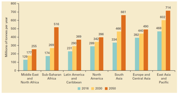
Canada is currently the world’s largest producer of MSW per capita. At slightly more than 36 metric tons per person per year, Canadians generate roughly 10 tons more MSW per person annually than the next highest garbage producers, Bulgarians and Americans (Tiseo, 2021). Summiting a list like this is obviously not in any country’s best interest—there are no kudos for reaching the top of the heap, so to speak. Is it therefore possible that those nations reaching the top will take the lead in reversing course?

Halifax is one Canadian city that apparently has. On August 1st, 2015, the city began providing a “green nudge” to citizens living in its urban core area with the introduction of the Clear Bag Policy, a policy designed to nudge households toward more responsible sorting of their waste, which, in turn, would result in an overall reduction in the total amount of waste generated. As Akbulut-Yuksel and Boulatoff point out, under the new policy, households were mandated to replace their black garbage bags, traditionally used for the disposal of their refuse, with clear, transparent bags. The Clear Bag Policy allowed households to put out the same number of garbage bags at the curb (six every other week), but all waste destined for the landfill was required to be disposed of in a clear bag (except for one dark bag permitted for privacy’s sake). This allowed waste collectors to screen and refuse any bags containing materials that should otherwise have been diverted from the landfill, such as recyclables, food waste, and hazardous waste. Clear bags also made apparent to everyone, neighbors and passersby alike, a given household’s waste-generation and disposal habits.^[33]

To test the Clear Bag Policy’s impact on a typical household’s generation of MSW, Akbulut-Yuksel and Boulatoff designed a quasi-experiment spanning the period from January 6, 2014, to July 28, 2017, with January 6, 2014, to July 31, 2015, serving as the pre-treatment period and August 1, 2015, to July 28, 2017, serving as the post-treatment period. MSW data collected during this time span included the weight (in tons) of weekly recycling and bi-weekly garbage generated by households within the urban core area. The authors adopted a “regression discontinuity” design that exploits the differences in total waste, recycling, and refuse amounts in the weeks preceding and following August 1, 2015. Results are depicted in the figure below.

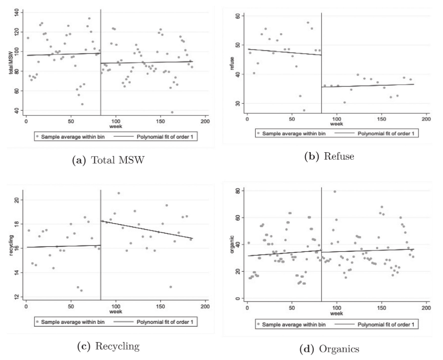
To begin, note that the vertical line in each panel (a)–(d) corresponds to the study’s 83rd week, the week of August 1, 2015 (when the Clear Bag Policy was implemented). In panels (a) and (b), we see statistically significant discrete drops at week 83 in total weekly MSW and landfilled refuse, respectively, generated by Halifax’s urban-core households—drops that are maintained for the remainder of the study period. In panel (c), we see a statistically significant increase in recycling; however, the increase occurring at week 83 is not maintained by the end of the study period. In panel (d), we see no statistical change in the amount of organic waste separated out for composting.

Akbulut-Yuksel and Boulatoff estimate that the Clear Bag Policy led to a 27% reduction in overall MSW, while increasing recycling by 15% compared to the pre-policy period. Their results also point to a short-term substitution effect between refuse and recycling (i.e., households became more responsible recyclers for a number of weeks after the policy was implemented). The authors found additional evidence suggesting that households located in neighborhoods with lower-than-average income and educational attainment exhibited larger improvements in their waste management and generation, thereby demonstrating that green nudges can affect household waste-management behavior differently across different socioeconomic groups. In the case of this particular study, the nudge exploited a household’s innate concern about its reputation as a waste generator, not unlike the reputational effect we learned about earlier with respect to the SmartAC program designed to prevent electricity blackouts in Southern California.

Promoting Energy Conservation

Speaking of descriptive and injunctive norms, Schultz et al. (2007) conducted a field experiment with approximately 300 households located in a California community in which different messages were tested in promoting household energy conservation. Each message (included with a household’s monthly energy bill) contained personalized feedback on the household’s energy usage in previous weeks. For those households randomly chosen to receive a descriptive-norm message (henceforth denoted D) that included information about average household usage in the household’s neighborhood for those previous weeks, the results were mixed. Households with higher-than-average usage reduced their energy usage while households with lower-than-average usage “boomeranged” by increasing their usage.^[34] The authors claim that the former result indicates the constructive power of social norms, demonstrating that normative information can facilitate pro-environmental behavior. The latter result demonstrates the potentially destructive power of social norms, demonstrating that a well-intended application of normative information can actually serve to decrease pro-environmental behavior. Of course, Homo economicus households with lower-than-average usage would have responded to the D message by decreasing their energy usage, not boomeranging to higher usage.

Alas, when an injunctive-norm message (I) was added to message D (henceforth denoted D+I) and sent to a separate, randomly chosen group of households—where social approval (indicated by a smiley face emoji) or disapproval (indicated by a frowning face emoji) was provided based upon the household’s usage relative to the neighborhood average—the boomerang effect disappeared. Hooray! Schultz et al. claim that this result demonstrates the potential reconstructive power of injunctive messages to eliminate the untoward effects of a descriptive norm. Homo sapiens households with lower-than-average usage just need a bit more nudging to reduce their energy usage.

The authors’ specific results (in the form of box plots) are presented in the figure below:

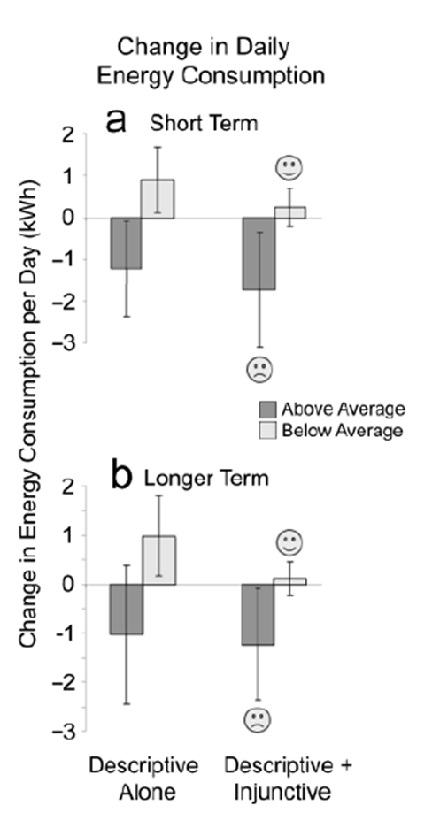
In this figure, Panel a presents results for the short term (where changes in usage are measured at the end of an initial one-week period) and Panel b for the long term (where changes in usage are measured at the end of a subsequent three-week period). The darker-shaded rectangles pertain to households with higher-than-average usage and the lighter-shaded rectangles pertain to households with lower-than-average usage. Further, the rectangles displayed on the left-hand sides of Panels a and b pertain to households that received message D, while the rectangles displayed on the right-hand side pertain to households that received message D+I. In cases where the segmented line  (i.e., the “whisker”) drawn through the middle of a rectangle does not extend beyond both the top and the bottom of the rectangle, the effect is considered statistically significant.

Hence, we see that, in the short term, households with higher-than-average usage who received the D message reduced their energy usage by a little over one kWh per day while households with lower-than-average usage increased theirs by a little under one kWh per day (this latter result demonstrates the boomerang effect). Also, in the short term, households with higher-than-average usage who received the D+I message again reduced their energy usage, this time by closer to two kWh per day. The D+I message provoked no statistically discernable effect on households with lower-than-average usage, thus eliminating the boomerang effect associated with the D message in the short term.

In the longer term, households with lower-than-average usage who received the D message continued using energy at an increased rate of roughly 1 kWh per day, but this boomerang effect was erased when the household received the D+I message. The short-term negative impact on households with higher-than-average usage who received the D message vanished over the longer term, but was sustained for households that had received the D+I message.

As with reducing environmental theft and littering, it seems that promoting energy conversation requires a well-targeted nudge.^[35]

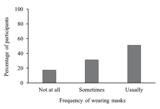
The authors found a powerful correlation between perception of the social norm and mask usage—conformity to the mask norm was the most influential determinant. Feeling relief from anxiety by wearing a face mask also promoted mask use. By contrast, frequency of mask usage depended much less upon the participants’ perceived severity of the disease and the efficacy of face masks in reducing infection risk, both for themselves and for others. These results lead Nakayachi et al. to conclude that effective nudging strategies against Covid-19 should appeal to social motivations among Homo sapiens such as the need to conform socially (at least as far as Japanese Homo sapiens are concerned). Further, the positive correlation between behavior and relieving anxiety by wearing face masks suggests that Homo sapiens consider subjective feelings rather than objective risks (i.e., when it comes to deciding the extent to which they will wear masks, Homo sapiens are prone to rely on an Affect Heuristic).

Text Messaging to Improve Public Health

We have seen previously how providing nudges in the form of targeted messaging can help reduce environmental theft and litter and help promote energy conservation. Might similar forms of messaging be used to improve health outcomes among people whose treatments require frequent and consistent self-administration of drugs? In a fascinating field experiment, Pop-Eleches et al. (2011) test whether short message service (SMS) text reminders sent via cell phone to roughly 430 patients attending a rural clinic in Kenya are effective in inducing adherence to antiretroviral therapy (ART) for the treatment of HIV/AIDS.

Patients older than 18 years of age who had initiated ART less than three months prior to enrollment were eligible to participate in the study. Participants received Nokia mobile phones and were informed by the researchers that some participants would be randomly selected to receive daily or weekly text messages encouraging adherence to their ARTs. The participants were also informed that one of their medications would be dispensed in bottles with electronic caps enabling the researchers to monitor daily usage.

Participants were randomly assigned to one of four treatment groups or to a control group that received no text messages. One-third of the sample was allocated to the control group, and the remaining two-thirds of the sample were allocated evenly to each of the four treatment groups. As Pop-Eleches et al. explain, the four text-message treatments were chosen to address the different barriers faced by ART patients such as forgetfulness and lack of social support. Short messages (translated as, “This is your reminder”) served as simple reminders to take medications, whereas longer messages (translated as “This is your reminder. Be strong and courageous, we care about you.”) provided additional support. Daily messages were close to the frequency of prescribed medication usage, whereas weekly messages were meant to avoid the possibility that the more-frequent daily text messages would habituate the participants. Hence, the four treatments are as follows: short daily message, long daily message, short weekly message, and long weekly message. The messages were sent at 12 p.m. rather than twice daily (during actual dosing times) to avoid excessive reliance on the accuracy of the SMS software.

Participants were expected to return to the clinic once a month according to standard procedures. The electronic bottle caps were scanned monthly by the pharmacy staff. ART adherence was calculated as the number of actual bottle openings divided by the number of prescribed bottle openings for a given treatment period. The researchers’ primary determinant of patient adherence to the ART was whether the patient adhered at least 90% of the time during each of four 12-week periods of analysis. A secondary determinant of adherence was whether patients experienced a treatment interruption exceeding 48 hours during each period of analysis.

Pop-Eleches et al. find that the fraction of participants adhering to their ARTs at least 90% of the time in the two treatment groups receiving weekly reminders is significantly higher than the fraction of those adhering in the control group. Likewise, members of the weekly-reminder groups are significantly less likely than those in the control group to experience at least one treatment interruption during the entire 48-week follow-up period. Such is not the case for the members of the daily-reminder groups. Both the fraction of participants adhering at least 90% of the time and the fraction experiencing at least one treatment interruption are not significantly different for those receiving daily reminders than those in the control group. Lastly, compared with the control group, neither the long- nor short-message groups are better at adhering to their ARTs at least 90% of the time. However, the long-message group experiences marginally fewer treatment interruptions than the control group.

Again, we find that Homo sapiens can be fickle when it comes to the specific wording of messages meant to nudge them toward better personal outcomes. And in this case, we see that the frequency with which they are exposed to the messaging can influence the extent to which Homo sapiens are ‘nudgeable.’ Pop-Eleches et al. conclude that increased frequency of exposure to a message can lead to habituation, or the diminishing of a response to a frequently repeated stimulus. More frequent messaging might easily cross the line of intrusiveness and thereby be more likely to be ignored.^[36], ^[37]

Invoking Fear as an Agent of Change

It has long been believed that information alone seldom provides sufficient impetus for Homo sapiens to change both their attitudes and actions (c.f., Cohen, 1957). The information must not only instruct the audience but must create motivating forces which induce attitudinal and behavioral change. Leventhal et al. (1965) identified the arousal of fear as one potential motivating force for change and set out to test this hypothesis in the context of a field experiment that provided subjects with information encouraging inoculation against tetanus bacteria.

Spoiler alert: The arousal of fear resulted in more favorable attitudes toward inoculation and the expression of stronger intentions among the experiment’s 60 subjects (who were seniors at Yale University) to get tetanus shots. However, actually taking action to get a shot occurred significantly more often among subjects who, in addition to having their fear aroused, also received information concerning a recommended plan of action to get the shot. Although actual decisions among subjects were unaffected by the fear factor in and of itself, some level of fear arousal was necessary for a subject to take action (i.e., to actually get inoculated). A recommended action plan was also not sufficient in and of itself for action to be taken by the subjects.

In Leventhal et al.’s study, fear-arousing and non-fear-arousing communications were used in recommending a clear action (getting a tetanus shot) which is 100% effective against contracting the disease. In addition, the perceived availability of a tetanus shot was experimentally manipulated by giving some subjects a specific plan to guide their action. It was hypothesized that subjects given a recommended action plan would choose to inoculate themselves at a higher rate. Most importantly, an interaction was anticipated between fear and action plan specificity: highly motivated subjects—that is, those exposed to the fear-arousing messages—were expected to show the greatest attitudinal and behavioral compliance with the messages when a clear recommended plan of action was also provided to them.

As part of the experiment, subjects were randomly provided with one of four booklets (i.e., enrolled in one of four treatments), with each booklet containing two sections: a “fear section” dealing with the causes of tetanus and including a case history of a tetanus patient, and a “recommendation section” dealing with the importance of shots in preventing the disease. There were two treatments in each section: “high fear” and “low fear” in the fear section, and “specific recommendation” and “non-specific recommendation” in the recommendation section.

The high-fear treatments were distinguished by “frightening facts” about tetanus (as opposed to “non-frightening facts” in the low-fear form), “emotion-provoking adjectives” describing the causes and treatment of tetanus (as opposed to “emotion-non-provoking adjectives”), and graphic photographs of a specific case history (as opposed to non-graphic photographs of the case history). The specific and non-specific recommendation treatments included identical paragraphs on the importance of controlling tetanus by inoculation and illustrated by statistics that clearly demonstrated that shots are the only powerful and fully adequate protection against the disease. In addition, both recommendations stated that the university was making shots available free of charge to all interested students. The specific recommendation also included a detailed plan of the various steps needed to get a tetanus shot.

Two types of responses were measured for each subject. Immediately after reading their booklets, subjects completed a questionnaire regarding their attitudes, feelings, and reactions to the experimental setting, as well as any previous inoculations. In addition, a record was obtained of all subjects taking a tetanus inoculation. The records were checked by student health authorities, and a count was made of the subjects in each treatment who were inoculated. The dates for inoculation were also obtained.

As previously mentioned in the spoiler alert, the high-fear treatments were very successful in arousing fear and its attendant emotions. Subjects reported feeling significantly greater fright, tension, nervousness, anxiety, discomfort, anger, and nausea in the high- as opposed to the low-fear treatment. During the four-to-six-week period between the experimental sessions and the end of classes, nine of the 60 eligible subjects went for tetanus shots. Of the nine, four were in the high-fear, specific-recommendation treatment; four in the low-fear, specific recommendation; one in the low-fear, non-specific treatment; and none in the high-fear non-specific treatment. Thus, all else equal, subjects in the specific-recommendation treatments were more likely to get inoculated while subjects in the high-fear treatments were apparently not.

To test whether specific recommendations were sufficient in and of themselves (without either low- or high-fear stimuli) to impel the subjects to inoculate themselves, Leventhal et al. formed a control group consisting of 30 subjects who were exposed solely to the specific recommendation. The procedures for contacting and inculcating subjects were identical to those used in the original four treatments. Not one of the subjects availed himself of the opportunity to obtain an inoculation. Thus, the authors conclude that a specific recommendation alone is insufficient to influence actions or attitudes.

Such is the story for inoculating against a disease such as tetanus. Does this result concur with the previous results obtained for reducing litter, environmental theft, drunk driving, and increasing energy conservation? Such is Homo sapiens’ varied responses to messaging.

Income Tax Compliance

In 1995 the Minnesota Department of Revenue (MDR) conducted a field experiment with 47,000 taxpayers (Coleman, 1996). The experiment tested alternative strategies to improve voluntary compliance with the state’s income tax laws, including (1) increased auditing of tax returns with prior notice to taxpayers, (2) enhanced tax preparation services provided to taxpayers, (3) descriptive norm messages contained in letters sent to taxpayers, and (4) introduction of a more user-friendly tax form. The primary measures used to evaluate compliance were (1) a taxpayer’s change in reported income between 1994 and 1995, and (2) a taxpayer’s change in state taxes paid between 1994 and 1995.

MDR uncovered three sets of key results:

1. Lower- and middle-income taxpayers facing an audit reported more income and paid more taxes.^[38] Increases were generally larger among taxpayers who had business income and paid estimated state taxes in 1993. Higher-income taxpayers had a mixed reaction to the threat of an audit—some responded positively, some negatively. The overall effect on their taxes was slight. Because they are expensive to conduct, audits are not particularly cost effective.
2. Enhanced tax-preparation services had no effect on reported income or taxes paid. Only 14% of taxpayers who were offered the expanded service availed themselves of it—slightly below the rate of taxpayers who had historically used traditional tax-preparation services at that time.
3. One of two messages contained in letters sent to taxpayers had a modest positive effect on reported income and taxes paid, which reinforces the argument that appeals to social norms increases responses. The letter read: “According to a recent public opinion survey, many Minnesotans believe other people routinely cheat on their taxes. This is not true, however. Audits by the Internal Revenue Service show that people who file tax returns report correctly and pay voluntarily 93% of the income taxes they owe. Most taxpayers file their returns accurately and on time. Although some taxpayers owe money because of minor errors, a small number of taxpayers who deliberately cheat owe the bulk of unpaid taxes (pages 5-6).”^[39]

In a subsequent experiment, Alm et al. (2010) sought to uncover the extent to which uncertainty in how much tax is owed correlates with tax evasion. In the experiment, subjects accrued tax on income earned during a simple task. Subjects could claim both tax deductions and tax credits. If a subject decided not to file a tax return, she paid zero tax but missed out on claiming a tax credit. In the experiment’s control group, subjects were made fully aware of the rules for claiming deductions and credits. In one treatment group, the uncertainty treatment, subjects had to guess the levels of deductions and credits they could claim. Only if they were audited would they learn how much tax they owed. In another treatment group, the information treatment, subjects had to guess how much income they should report to the tax authority, but they could press a button to learn exactly how much they should report. As expected, the authors found that both the filing and compliance rates were highest (although only slightly) among subjects in the information treatment. Similar to the provision of enhanced tax-preparation services in the MDR study, it appears that providing additional information on how much income to report on their tax returns does not, all else equal, compel the typical Homo sapiens taxpayer to comply with their taxpaying obligations.^[40]

The Not-So-Good Samaritan

It is helpful to know that the Judeo-Christian parable of the Good Samaritan has value in suggesting both personality and situational variables relevant to helping others. At least that is the conclusion reached by Darley and Batson (1973) in their innovative experiment with seminary students roughly 50 years ago. Using the Good Samaritan parable as their motivation, the authors presented the unwitting students with surprise, real-life encounters with a person in apparent distress and studied the students’ responses. Surprisingly, a student’s personality (or disposition) was unable to predict whether he would stop and offer assistance. In contrast, the extent to which a student was in a hurry as he came upon the person needing assistance (i.e., the situation) could explain the student’s response—those in more of a hurry were less likely to stop and offer assistance.

The parable, which appears in the Gospel of Luke (Luke 10: 29-37 RSV), offers insight into the roles that both dispositional and situational effects are expected to play in summoning assistance from a passer-by:

“And who is my neighbor?” Jesus replied, “A man was going down from Jerusalem to Jericho, and he fell among robbers, who stripped him and beat him, and departed, leaving him half dead. Now by chance a priest was going down the road; and when he saw him he passed by on the other side. So likewise a Levite [priest’s assistant], when he came to the place and saw him, passed by on the other side. But a Samaritan, as he journeyed, came to where he was; and when he saw him, he had compassion, and went to him and bound his wounds, pouring on oil and wine; then he set him on his own beast and brought him to an inn, and took care of him. And the next day he took out two dennarii and gave them to the innkeeper, saying, “Take care of him; and whatever more you spend, I will repay you when I come back.” Which of these three, do you think, proved neighbor to him who fell among the robbers? He said, “The one who showed mercy on him.” And Jesus said to him, “Go and do likewise.”

As Darley and Batson point out, the Samaritan can be interpreted as responding spontaneously to the situation rather than being preoccupied with the abstract ethical or organizational do’s and don’ts of religion as we might expect the priest and Levite to be. Hence, to the extent that the parable is relevant in the modern age, we should expect Homo sapiens to share more the disposition and situation of the Samaritan than that of the priest or priest’s assistant to stop and offer assistance to someone in distress. Further, it is clear from the parable that the Samaritan had ample time on his hands to provide assistance. After binding the man’s wounds, pouring on oil and wine, bringing him to an inn, and continuing to administer care there, the Samaritan still promised to return the next day to check up on the man’s recovery. This suggests that the Samaritan was not in a hurry at the time, and therefore his situation was even more amenable to stopping and offering assistance.

Darley and Batson coalesce these interpretations into three testable hypotheses, the first two of which correspond to situational effects and the third corresponding to dispositional effects:

1. Homo sapiens who encounter a situation possibly calling for a helping response while thinking religious and ethical thoughts will be no more likely to offer aid than persons thinking about something else.
2. Homo sapiens encountering a possible helping situation when they are in a hurry will be less likely to offer assistance than those not in a hurry.
3. Homo sapiens who are religious in a Samaritan-like fashion will offer assistance more frequently than those religious in a priest- or Levite-like fashion.

To test these hypotheses, the authors recruited 40 students at Princeton Theological Seminary to participate in a two-part field experiment. In the first part of the experiment, each subject was administered a personality questionnaire in order to identify the subject’s respective “religiosity” type (e.g., whether a subject viewed religion as more a “means to an ends” in life, an “ends in itself,” or as a “quest for meaning” in the subject’s personal and social world—which is commonly believed to represent the Good Samaritan’s religiosity). In the experiment’s second part, the subject began experimental procedures in one building on campus and was then asked to report to another building for later procedures. While in transit, the subject passed a slumped “victim” planted in an alleyway. Unbeknownst to the student, measurements were taken of the degree to which he stopped and provided assistance to the victim.^[41] Prior to being in transit, the student was told to hurry (at varying levels of admonition) to reach the other building. The student was also told the topic of a brief talk he was to give to a waiting audience after arriving at the other building. Some students were instructed to give a talk on the jobs in which seminary students would be most effective while others were instructed to give a talk on the parable of the Good Samaritan.

Darley and Batson found that subjects in more of a hurry (based upon the degree of admonishment provided by the experimenters) were (1) less likely to stop and offer assistance, but (2) once they stopped, less likely to offer less help than were subjects in less of a hurry. Whether the subject was going to give a speech on the parable of the Good Samaritan or job prospects for seminary students, it did not significantly affect his helping behavior in either of these two respects. These results confirm both Hypotheses 1 and 2. Regarding Hypothesis 3, the authors claim that religiosity played no role in either respect—either choosing to stop, or once stopped, choosing to provide a higher level of assistance.^[42]

These results are suggestive of the motivations driving Homo sapiens to stop and assist strangers in distress. But this leaves the question unanswered as to what might motivate Homo economicus to provide assistance. Presumably, Homo economicus would be capable of reading the victim’s circumstances well enough to make a calculated, rational decision to stop or not, and if having chosen to stop, then how much assistance to provide. Sounds a bit scary if you ask me.

Toxic Release Inventory

In Chapter 8 we considered a game where providing one of two players with additional information about a certain facet of the game ultimately led to a perverse outcome—a reduction in the player’s payoff. This result was considered counterintuitive, particularly from the perspective of Homo economicus who, according to the rational-choice model, is never supposed to be made worse off when more information is made available. Presuming that Homo sapiens could in fact be made better off through the provision of additional information, the US government fostered a natural experiment to test this hypothesis with respect to improving the country’s natural environment via the public provision of its data on the levels of toxins emitted by every permitted company in the country. To this day, emissions are self-reported by the polluters, compiled by the Environmental Protection Agency (EPA), and then made publicly available. The EPA inspects approximately 3% of firms per year; one-third of regulated facilities fail to comply with reporting requirements each year.

According to Fung and O’Rourke (2000), between the Toxic Release Inventory’s (TRI’s) inception in 1988 and 1995, releases of chemicals listed on the TRI declined by 45%. Results are depicted in the figure below where—measured as a percentage of emissions in 1989—the emissions of chemicals included in the TRI diminished steadily over the next five years relative to the emissions of pollutants not included in the TRI.

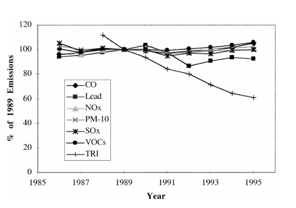
The authors argue that the TRI achieved this regulatory success through the mechanism of ‘‘populist regulation,’’ by establishing an information-rich context for private citizens, interest groups, and firms to solve environmental problems. Armed with the TRI, community, environmental, and labor groups can take direct action against the worst polluters, spurring them to adopt more effective environmental practices. Further, the TRI catalyzes popular media campaigns encouraging state-level environmental agencies to enforce regulations against egregious polluters. Additional research also suggests that publicity tied to the government’s sharing of TRI data has a negative impact on stock prices of publicly traded firms listed in the TRI. Apparently, Homo sapiens from various walks of life are making use of this information to help clean up their local environments; they have been nudged simply via the provision of information in a conveniently accessible database provided by the EPA.

Reducing Drunk Driving

In 2002, Montana ranked first in the nation in alcohol-related fatalities per vehicle miles traveled. Twenty-one to thirty-year-olds (young adults) represented nearly half of all alcohol-related crashes. Perkins et al. (2010) evaluated the efficacy of a high-intensity, descriptive social-norms marketing media campaign aimed at correcting normative misperceptions about drunk driving, and thereby reducing drinking-and-driving behavior among young adults. Over a 1½ year period, participating counties in the state experienced a “high-dosage” media campaign while non-participating counties experienced a “low-dosage” version.

The social norms media campaign consisted of television, radio, print, and theater ads in addition to posters and promotional gifts. Ads appealed to traditional social norms. For example, one television commercial depicted a typical Montana ranch family in a barn preparing to ride horses. As Perkins et al. report, the script read:

In Montana, our best defense against drinking and driving is each other. Most of us prevent drinking and driving. We take care of our friends, our families, and ourselves. Four out of five Montana young adults don’t drink and drive. Thanks for doing your part.

Another TV ad depicted a ski lodge window with snow falling. A male voice read the script:

In Montana, there are two things you need to know about snow: how to drive on it and how to ski on it. After a day on the slopes and some time in the lodge, my friends and I all take turns being designated drivers.” The view widens to reveal the message written on the window, “Most of us (4 out of 5) don’t drink and drive.” The commercial closes with the voice asking, “How are you getting home?

One of the posters used in the marketing campaign is depicted below:

The high dosage media campaign ran for 15 months from January 2002 to March 2003. Because many of the intervention counties are sparsely populated (e.g., six are home to fewer than 600 persons in the 21–34-year-old range), Perkins et al. placed a heavy focus on television airtime since not all newspaper and radio advertisements could effectively reach the entire target audience. A total of 18 media advertisements (i.e., 9 television and 9 radio) were used. Social norms advertisements consistently emphasized positive behavior and avoided negative and/or fear-based messages. The television ads were aired during two media flights. The first lasted five and a half months while the second lasted six months. The two radio flights lasted six and a half and six months, respectively.

Television and radio ads were supplemented by local and college newspaper advertisements, theater slides, billboards, various print and promotional items (i.e., t-shirts, key chains, pens, and windshield scrapers), and indoor advertisements. These additional advertisements and theater slides ran from January 2002 through December 2003. Over 250 print ads were taken out in local and college newspapers, 70 theater slides appeared on over twenty movie screens, and a billboard design appeared in seven locations for a two-month period. Over 45,000 promotional items were distributed in the intervention counties. Lastly, 41 indoor ads were placed in Bozeman and Missoula restaurants, which were the two cities with the largest number of individuals from the target population.

The authors measured exposure to the media campaign using both prompted and unprompted recall. Survey participants were asked, “During the last twelve months, do you remember seeing or hearing any alcohol prevention campaign advertisements, posters, radio or TV commercials, or brochures?” If they responded yes, then they were asked what the main message was that they remembered. Participants’ perceptions of others’ behavior were assessed with two questions: (1) “During the past month, do you think the average Montanan your age has driven within one hour after consuming two or more alcoholic beverages within one hour?”, and (2) “In your opinion, among Montanans your age who drink, what percentage almost always make sure they have a designated non-drinking driver with them before they consume any alcohol and will be riding in a car later?”

Lastly, to measure their personal behavior before and after the campaign, survey participants were asked, “During the past month, have you driven within one hour after you have consumed two or more alcoholic beverages within an hour?”, and “When you consume alcohol and know that later you will be riding in a car, what percent of the time do you make sure you have a designated non-drinking driver with you before you start drinking?” In addition, participants were asked, “The current law in Montana states that a blood alcohol concentration (BAC) of above 0.10% constitutes legal impairment. Would you support or oppose changing the law in Montana to make a BAC above 0.08% constitute legal impairment? This change would permit less alcohol consumption before driving.”

Perkins et al.’s results are presented in the following table:

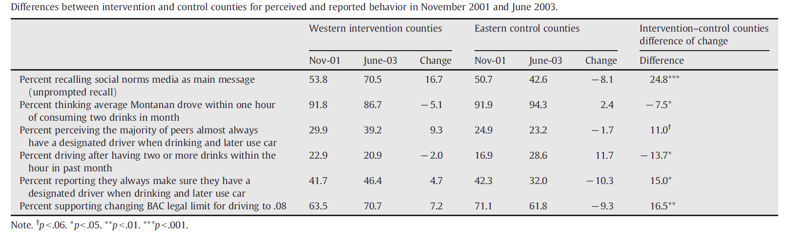
The first row of the table presents results for social-norms message recall by participating (or intervention) and non-participating (i.e., control or non-intervention) counties prior to and following the media campaign. As shown in the last column for this row, the campaign was successful at differentially exposing Montanans between the ages of 21 and 34 to social norms messages (the statistically significant difference in message recall across intervention and control counties is 16.7% – (-8.1%) = 24.8%). In the table’s second row, we see that the social-norms campaign reduced misperceptions of those in the intervention counties relative to those in the control counties, such that those in the intervention counties believed the average Montanan their same age had driven less often within one hour of consuming two or more drinks in the past month compared to those in the control counties. Similar results were found in the table’s third row regarding the perception of peer use of designated drivers. Participants in the intervention counties believed that the majority of Montanans their age almost always have a designated driver with them when they consume alcohol and would be riding in a car later, significantly more so than those in the control counties. As the authors point out, these combined findings suggest that the campaign was successful at reducing normative misperceptions regarding peer drinking and driving behavior.

Relative to participants in the control counties, Perkins et al. find that the percentage of young adults in the intervention counties who reported driving within an hour of consuming two or more drinks in the previous month decreased following the social norms campaign. In contrast, the percentage of young adults in the control counties who reported driving within an hour of consuming two or more drinks in the previous month actually increased during this time. With reported driving after drinking decreasing in the intervention counties by 2% and increasing in the control counties by 12%, there was an overall statistically significant decrease in the intervention counties compared to the control counties of almost 14%.

Similarly, the percentage of individuals in the intervention counties who reported that they always use a designated driver if they plan to drink increased following the social norms campaign, whereas there was a drop in the use of designated drivers in the control counties, resulting in an overall increase in the use of designated drivers in intervention counties relative to the control counties of 15%. Lastly, results indicate that participants in the intervention counties increased their support for changing the BAC legal limit for driving to 0.08 following the social norms campaign, which is a significant difference compared to the decrease in support seen among participants in the control counties. The authors conclude that the social-norms media campaign was effective at reducing high-risk drinking-and-driving behavior and increasing use of protective behaviors (i.e., designated drivers) among those in the intervention counties compared to those in control counties.

If these findings were not enough, Perkins et al. also obtained archival motor vehicle crash records from the intervention and control counties. The authors point out that the data do not provide a perfect test of the intervention’s impact because crashes in Montana were coded as alcohol-related when anyone involved in the crash was under the influence of alcohol, regardless of who was driving or at fault. Moreover, the available data only recorded if an alcohol-related crash occurred in the county and not if the driver was from that county. Hence, there may have been some blurring across county lines which, nevertheless, would serve to reduce an observed impact of the intervention (i.e., it would bias the impact of intervention downward). Nevertheless, in spite of these qualifications, the data revealed a pattern in the expected direction. In 2001 there were 9.6% and 10.1% alcohol-related crashes in the intervention and control counties, respectively. However, the difference was not statistically significant. In 2003, after the social-norms media campaign, alcohol-related crashes had declined to 9.1% in the intervention counties and had risen to 10.3% in the control counties, resulting in a statistically significant difference between the two types of counties.

In conclusion, the authors argue that the results of their study provide strong evidence that a comprehensive social-norms media campaign can affect normative perceptions and drinking behavior among young-adult Homo sapiens, at least in terms of nudging them away from drinking and driving.

Increasing Voter Turnout

In a field experiment conducted a month before the 1984 US presidential election, a treatment group of Ohio State University students contacted by telephone was asked to predict whether they would register to vote and whether they would actually vote in the coming days (Greenwald et al., 1987). All students in the treatment group predicted that they would vote, and larger numbers of these students actually registered to vote and voted in comparison with uncontacted students in a control group.

In what Greenwald et al. labeled Experiment 1, a larger percentage of students in the treatment group (who received the simple nudge of a question posed over the phone) registered to vote than did students in the control group (who received no phone call) (20.8% to 9.1%). However, this difference was not statistically significant. To the contrary, the difference in actual voting between the two groups of students (86.7% versus 61.5%) was statistically significant.

In the US, groups like Rock The Vote and Nonprofit VOTE promote a host of different ways to nudge prospective voters to the polls. As Greenwald et al.’s field experiment has shown, it does not really take a big nudge to move the needle on voting. Of course, this is not to say that public calls by some groups to make presidential election day a national holiday, move voting day from the first Tuesday to the first Saturday in November, or move to mail-in voting, are not without merit.

Cultural Conflict and Merger Failure

Recall Camerer and Knez’s (1994) findings from their laboratory experiments involving mergers in the context of the Weakest Link game. Merged groups obtained inefficient equilibria more frequently than did the separate smaller groups of which the respective merged groups were comprised, suggesting that mergers can exacerbate an extant inefficiency problem in games where inefficient equilibria are focal points, if not the consequence of dominant strategies.

In a novel field experiment, Weber and Camerer (2003) tested for the efficiency effects of mergers by engaging participants in a guessing game similar to Charades. Every subject was shown the same set of 16 photographs, each depicting a different office environment. While most of the photographs shared some common elements (e.g., people, furniture, room characteristics, and so forth), each photograph was unique with respect to the number of people and their characteristics (e.g., gender, clothing, ethnicity), physical aspects of the room (e.g., high ceilings, objects on walls, furniture), and the people’s actions (e.g., conversing with others in the picture, talking on the telephone, working at a computer).

Subjects were paired. The experimenter then presented 8 of the 16 photographs in a specific order to only one of the two subjects who had been randomly assigned to play the role of the manager. The manager then described the eight photographs any way she liked to the other subject who, by default, was playing the role of employee. The employee’s goal was to select the correct 8 photographs from his collection of the 16 in the same order as presented by the manager as quickly as possible. Each pair of subjects repeated the task for 20 rounds, with the subjects alternating roles of manager and employee each round and the experimenter randomly selecting another set of eight photographs with which to play.

Then two pairs were randomly merged together. One of the pairs was designated “acquiring firm,” and one member of this firm was chosen as manager of the now “merged firm” for the remainder of the experiment. The other member of the acquiring firm was designated as an employee, and one member of the “acquired firm” was also selected randomly as an employee. The other member of the acquired firm was now finished participating in the experiment. In the end, therefore, each merged firm consisted of one manager and two employees. Henceforth, the manager played the same game simultaneously with both employees for 10 rounds. However, now each employee completed his or her identification task with the manager independently of the other employee. Each employee tried to guess the eight photographs as quickly as possible. The manager’s goal was to achieve the lowest possible average guessing time across the two employees.

As Weber and Camerer point out, the identification task created simple cultures by requiring subjects to develop conversational norms enabling quick reference to the photographs. For instance, one pair of subjects began by referring to a particular picture as “The one with three people: two men and one woman. The woman is sitting on the left. They’re all looking at two computers that look like they have some PowerPoint graphs or charts. The two men are wearing ties and the woman has short, blond hair. One guy is pointing at one of the charts” (p. 408). After several rounds, this group’s description of the picture had become condensed to simply “PowerPoint.”

The study’s specific results are presented in the following figure:

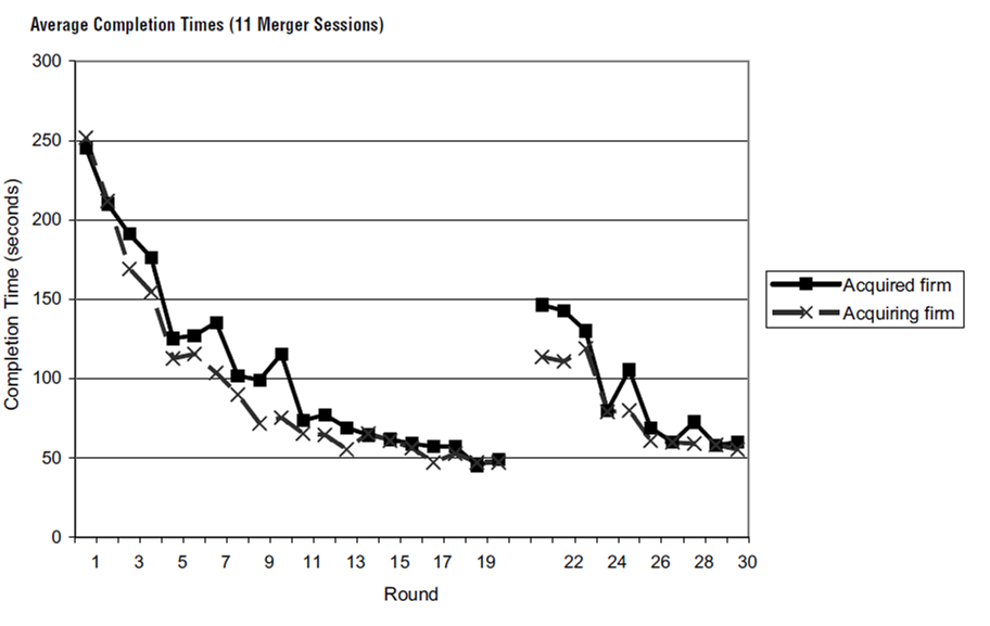
First, note that the average completion time is initially high for the single pairs (what were later to become the acquiring and acquired firms), with both pairs requiring roughly four minutes (250÷60) to complete their tasks in the first round. Average times fell steadily over time as the pairs developed a common language, eventually reaching less than a minute by the 20th round of the experiment. Immediately after the merger (in what is effectively round 21 in the figure), the merged firm performed better than the original pair groups did initially.^[43] But relative to where the original pairs ended in round 20 and where the merged firm began, there is a noticeable decrease in the merged firms’ performances—from two (acquiring firm) to two and a half (acquired firm) minutes on average for the merged firm compared to less than a minute for the original pair groups. And in the end, the average merged firm never attains the same level of performance as the average original pair.

Surely these results are a rough representation of how mergers actually transpire between acquiring and acquired firms. After all, Homo sapiens are a gregarious species. To the extent that management can harness and channel this gregariousness, it could very well be that the merged firm’s efficiency is enhanced rather than impeded after the merger (as Weber and Camerer’s results suggest). Recall that in the experiment, the employees of the merged firm made their guesses independently of each other. Perhaps if they could have worked together, their overall times would have been reduced sooner and, ultimately (at the end of the tenth round), improved vis-à-vis the original pair times. Either way, it is unclear whether Homo economicus subjects could have performed any better in this experiment.

Messy Work Space

In his entertaining book, Messy: The Power of Disorder to Transform Our Lives, author Tim Harford explains the multitude of settings in which we Homo sapiens are better served by resisting the temptation to tidily organize our lives, particularly in our professional settings (Harford, 2016). Rather, a certain degree of messiness nourishes our creative instincts and often leads to greater productivity. Harford provides several examples, from musicians Brian Eno’s, David Bowie’s, Miles Davis, and Keith Jarrett’s “messy” abilities to improvise and embrace randomness; to Martin Luther King Jr.’s willingness to go off-script in his most famous “I Have a Dream” speech; to the spontaneous, self-deprecating humor of Zappos customer service reps; to the daring battlefield maneuvers of General Rommel; to Amazon founder Jeff Bezos’ counterintuitive business strategy; to world chess champion Magnus Carlsen’s puzzling chess moves; to the nomadic, freewheeling methods of scientists Erez Aiden and Paul Erdős, and the eclectic and messy collaborations among the scientists inhabiting Building 20 on the campus of the Massachusetts Institute of Technology (MIT) during the last half of the 20th century. In each case, it was the messiness of the individual’s or group’s method that helped empower their sense of self and, ultimately, motivate their success.

In one particular study cited by Harford, authors Knight and Haslem (2010) designed a field experiment to measure the extent to which office workers’ freedom to customize, or mess, their workspaces—and thus, empower themselves—impacts their wellbeing (i.e., feelings of psychological comfort, organizational identification, physical comfort, and job satisfaction, as well as their overall productivity).^[44] As the authors point out, companies have traditionally believed that lean, open, uncluttered office spaces are efficient. These types of spaces can accommodate more people and thus, exploit economies of scale. Desks can also easily be reconfigured for use by other workers. As a result, space occupancy can be centrally managed with minimal disruptive interference from workers. Surprisingly, there is a lack of empirical evidence to support these claims.

To the contrary, some organizations have sought to enrich their workspaces by investing in “environmental comfort” (e.g., aesthetically pleasing artwork and living plants) to enhance the physical and mental health of their employees. And some of these organizations go even further by encouraging employees to decorate their personal workspaces with meaningful artifacts to project their identity onto their environment and to give some sense of permanency, control, and privacy. In this respect, these organizations encourage their employees to messy their workspaces.

Given this dichotomy between “lean” and “enriched” workspaces, Knight and Haslem designed a field experiment to directly test the hypotheses that empowering workers to manage, and have input into, the design of their workspace enhances their sense of organizational identification, emotional well-being, and productivity. Four separate office spaces were designed for the experiment: (1) a lean, minimalist office space intended to focus the employee’s attention solely on the work at hand (in particular, through the imposition of a clean desk policy), (2) an enriched office space incorporating art and plants, but where the employee has no input into their arrangement, (3) an empowered office space that allows an employee to design her office environment using a selection of the same art and plants as in the enriched office space, but allows her to realize something of her own identity within the working space, and (4) a disempowered office space where the employee’s workspace design in the empowered office is overridden by the experimenter so that an initial sense of autonomy within the workspace is effectively revoked.

In the experiment, 112 men and women ranging in age from 18 to 78 years were randomly assigned to one of the four office space types.^[45] The laboratory office was a small interior office measuring 3.5m x 2m. The office had no windows or natural light. At the outset of the experiment, each participant was left alone in the office space for five minutes to take in the ambient environment. The office contained a rectangular desk and a comfortable office chair. The room was lit by diffused, overhead fluorescent tubes, the floor was carpeted, and an air conditioning system kept the room at a constant temperature of 21 °C.

In the lean office, no further additions to the room were made. In the enriched office, six potted plants had already been placed toward the edge of the desk surface, so as not to impinge on the participants’ working area. Six pictures were hung around the walls. The pictures were all photographs of plants enlarged onto canvas. In the empowered office, the pictures and plants had been placed randomly around the room. Participants were told that they could decorate the space to their taste using as many, or as few, of the plants and pictures provided. They could, therefore, work in a lean or very enriched space or at a point anywhere along that continuum. The disempowered office was the same as the empowered office; however, when the experimenter re-entered the office, she looked at the chosen decorations, briefly thanked the participant, and then completely rearranged the pictures and plants, thereby overriding the participant’s choices. If challenged, participants were told that their designs were not in line with those required by the experiment.

After getting situated in their offices, participants were instructed to perform a card-sorting task. Three packs of playing cards had been shuffled together, and the participant was required to sort them back into the three constituent packs and then to sort each pack into its four suits (hearts, clubs, diamonds, and spades). These suits then had to be ordered from ace to king and placed in discrete piles, leaving 12 piles in total. The key performance measures were the time taken to complete this task and the number of errors made.

The participants were then asked to perform a second “vigilance task,” whereby they were given a photocopy of a magazine article and asked to cross out and count all the lowercase letters “b” that were on the page. The time taken to complete the task was measured as well as the number of errors (missed b’s). After completing this task, the participants completed a 74-item questionnaire, answering questions that would enable the researchers to test the previously mentioned hypotheses.

Knight and Haslem found that the average participant performed the card sorting task best in the empowered office space. When measured in minutes to complete the task, the results (i.e., the measured productivity differences between the lean, enriched, empowered, and disempowered offices) are statistically different for two of the study’s three main hypotheses – the first two hypotheses (H1 and H2, respectively) that the empowered office inspires the highest productivity level (particularly when compared with the enriched office) are confirmed. Regarding the vigilance task (measured in minutes to complete the task), the average participant again performs best in the empowered office; interestingly, the disempowered office space is associated with a particularly deleterious effect on productivity. In terms of total productivity measured in minutes to completion across the two tasks, the empowered office environment inspires the most productivity, while the disempowered office space inspires less productivity vis-à-vis the enriched office space.

With respect to the more intangible effects on well-being and organizational identification, the typical participant’s sense of involvement, autonomy, and psychological comfort ranked highest in the empowered office space, particularly in the enriched office space. Regarding one’s sense of identification with the organization (in this case, the field experiment’s various tasks), the only statistically significant effect occurred in the disempowered office. Disempowerment resulted in a decrease in organizational identification.

The message from Knight and Haslem’s field experiment seems clear. Empowering office workers, which, from the perspective of managers, risks introducing a degree of messiness into workspaces, can result in greater productivity and a sense of well-being among employees. Empowerment does come with a risk though. Once the empowerment genie is out of the proverbial bottle, woe to the manager who tries to stuff it back in.

Messy Traffic Crossing

Given Homo sapiens’ predisposition for all things tidy, one can be forgiven for concluding that Dutch traffic engineer Hans Monderman had lost his mind when he argued that traditional traffic-safety infrastructure—warning signs, traffic lights, metal railings, curbs, painted lines, speed bumps, etc.—is often unnecessary and, worse, can endanger those it is meant to protect. Yet according to Vanderbuilt (2008), this was indeed Monderman’s sentiment, based as it was upon the Dutch traffic guru’s simple axiom, ‘when you treat people like idiots, they’ll behave like idiots.’ To wit, Monderman devoted the better part of his career designing roads to feel more dangerous (yes, “more”) so that pedestrians and drivers would navigate them with greater care (Vanderbuilt, 2008).^[46]

As recounted by Vanderbuilt, Monderman’s most memorable design was built in the provincial Dutch city of Drachten in 2001. At the town center, in a crowded four-way intersection called the Laweiplein, Monderman removed not only the traffic lights but virtually every other traffic control. Instead of a space cluttered with poles, lights, “traffic islands,” and restrictive arrows, Monderman installed a radical kind of roundabout (which he called a squareabout because it resembled more a town square than a traditional roundabout) marked only by a raised circle of grass in the middle, several fountains, and some very discreet indicators of the direction of traffic, which were required by law. Rather than creating clarity and segregation, Monderman had created confusion and ambiguity in the minds of drivers and pedestrians. Unsure of what space belonged to them, drivers became more accommodating and communicative. Rather than give drivers a simple behavioral mandate—say, a speed limit sign or a speed bump—Monderman’s radical design subtly suggested the proper courses of action.

A year after its redesign, the results of this extreme makeover were striking. According to Euser (2006), not only had congestion decreased in the intersection—buses spent less time waiting to get through the intersection, for example—but there were half as many accidents even though total car traffic had increased by a third. Further, both drivers and, unusually, cyclists were signaling more often. Despite the measurable increase in safety, local residents perceived the squareabout to be more dangerous.

Roughly five years after the redesign, Euser found that on the busiest street entering into the squareabout, the average waiting times for automobiles had dropped from 50 to about 30 seconds. Waiting times for public buses dropped from over 50 seconds to 26 seconds heading in one direction and to 38 seconds heading in the other. The number of cyclists entering the intersection between 3:30 pm and 5:30 pm on a typical day and signaling with their left hands increased from roughly 50% to 80%, while the percentage of right-hand signaling increased from 9% to 47%. Underscoring these changes in waiting times and cyclist behaviors, the number of cyclists accessing the intersection in the same two-hour timeframe on a typical day had increased by roughly 5% since 2000. The number of “person car units” (PCUs) entering the intersection during the typical evening rush hours had increased by roughly 30%. Three years after the squareabout’s construction, the total number of traffic accidents had been roughly cut in half.

In surveys conducted with Drachten residents both before and after construction of the squareabout, traffic was generally considered less safe, particularly among the elderly. Motorists and cyclists reported feeling less safe, while there was no discernable change in the perceived safety of pedestrians. In terms of the Laweiplein’s spatial quality, survey respondents generally reported experiencing an improvement. In general, bus drivers reported feeling positive about the new design, in particular, that their wait times had improved.

Though Monderman’s squareabout may be counterintuitive and revolutionary, clearly the change in Homo sapiens’ traffic behaviors it has impelled is yet another indication of Homo sapiens’ susceptibility to nudges which, in this case, involves the redesign of existing infrastructure.^[47] As for Homo economicus, whose rational mind is enthralled by tidiness and order, navigating the squareabout is something she would never allow herself to get used to.

Disorganized Pedestrians

I don’t know about you, but in my daily life I suffer from what might be called myriad “micro-inefficiencies.” I waste minutes each day searching for things—my cellphone charging cable, my glasses, keys. And then, I fumble with these things once I have found them—extricating the charging cable from its little stuff sack, fishing my keys out of my pocket, taking my glasses off to see something up close and then forgetting where I left them. These micro-inefficiencies add up over a lifetime, perhaps claiming a year or more off my lifespan.

Living in a small town, I am also fortunate to benefit from certain “micro-efficiencies.” No matter where I travel in town or the surrounding valley, I rarely encounter congestion, whether on the road walking, riding my bicycle, driving my car, walking or jogging on a sidewalk, or waiting in line at a restaurant or the grocery store checkout. So, in many respects, I should not complain about my micro-inefficiencies. This is especially the case when I travel to busier cities—the traffic congestion in Salt Lake City and Seattle never ceases to amaze and humble (okay, and often frustrate) me. I also experience similar feelings of amazement, humility, and frustration when walking the bustling New York City sidewalks in midtown Manhattan in and around Grand Central Station.

As a visitor to the city, I am inclined to gawk at the buildings, the street life, and the captivating mix of other pedestrians. At the same time, I am tasked with having to navigate the sidewalks without bumping into or impeding the flow of other pedestrians. The flow of pedestrians in this section of New York City might best be described as organized disorganization. It is as if we Homo sapiens tacitly and instinctively coordinate to reduce what would otherwise result in more substantial micro-inefficiencies in our lives. Like fish schooling in the oceans and birds flocking in the sky, New York City pedestrians self-organize to reduce the incidence of collision. As Murakami et al. (2021) point out, pedestrians’ instantaneous decisions are influenced more by anticipated future positions rather than the current positions of their nearest neighbors, which suggests that crowded pedestrians are not just passively repelled by other pedestrians, but actively discern passages through a crowd by anticipating and tacitly negotiating with neighbors to avoid collisions in advance.

To test the sensitivity of these tacit negotiations, Murakami et al. conducted a simple field experiment of lane formation, where some participants walked while using their cellphones, thus potentially interfering with their ability to anticipate neighbors’ motions. Two groups of 27 pedestrians each voluntarily agreed to walk in bidirectional flows in a straight mock corridor. Three participants in one of the two groups were visually distracted by using their cellphones to potentially disrupt their anticipatory interactions with the other pedestrians in both their group and the other group. This situation is depicted in panel A of the figure below. The three circled individuals with yellow hats are looking at their cellphones as they move with the other yellow-hatted pedestrians from left-to-right in the corridor. The red-hatted pedestrians are all moving right-to-left.

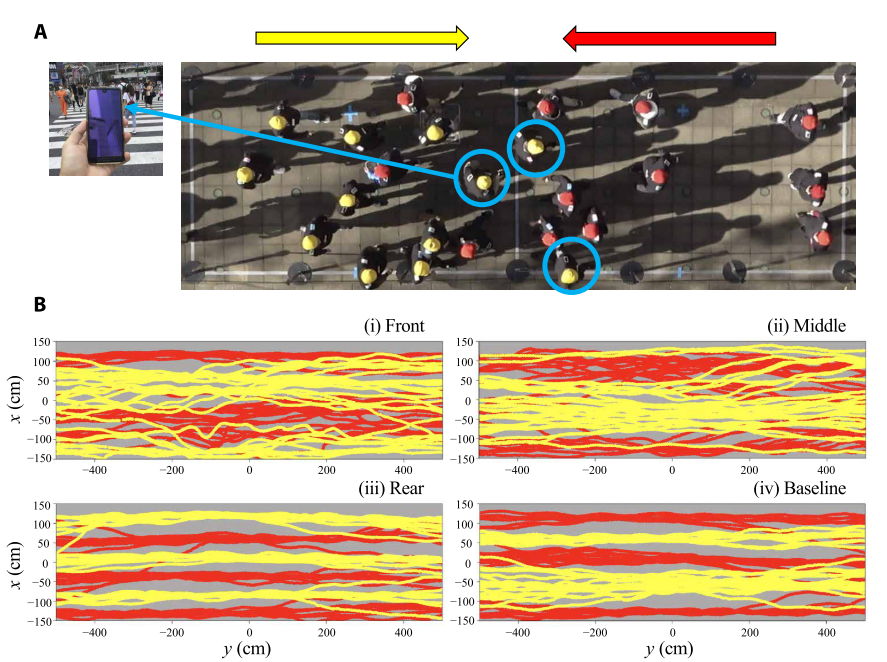
The authors hypothesized that distracted pedestrians located in the front of their group, directly facing the oncoming crowd, would have the most influence on overall crowd dynamics. To test this, Murakami et al. designed three treatment scenarios. In one treatment, the three randomly selected cellphone users were positioned at the front of their group (front treatment), while in the other two treatments three randomly selected cellphone users were placed in the middle (middle treatment) and rear (rear treatment), respectively, of their group. In a control scenario, no one was selected to use their cellphone. The experiments were replicated 12 times for each of the treatment and control scenarios.

The authors found that pedestrians participating in the front treatment were significantly slower than those participating in the control scenario, suggesting that distracted participants in the front condition influenced overall pedestrian flow as expected (i.e., the three distracted pedestrians created a micro-inefficiency for the other pedestrians). This inefficiency is depicted by the preponderance of red and yellow overlapping squiggly lines in the above figure’s graph (i) of panel B relative to the absence of overlapping squiggly lines in graph (iv). However, pedestrians participating in the middle and rear treatments were not found to be significantly slower than participants in the control scenario (depicted by comparing graphs (ii) and (iii) with graph (iv) in the figure).

Just for fun, check out these videos of the experiment. The first video is of the control scenario, where no pedestrians are looking at their cell phones:

The second video shows the front treatment, where the three cell phone users are located at the front of the red-hatted group of pedestrians walking left-to-right:

The third and fourth videos are of the middle and rear treatments. In the middle treatment, the three cellphone users are located in the middle of the yellow-hatted group walking right-to-left, and in the rear treatment, the three cellphone users are located at the rear of the red-hatted group walking left-to-right.

Beneficial Biases in Strategic Decision-Making

Are Homo sapiens who start their own small businesses (i.e., entrepreneurs) fundamentally different from those who choose to work in larger, more-established businesses (i.e., managers)? This question has spurred a long line of research concerning the mindset and behavior of entrepreneurs, with findings suggesting that entrepreneurs are risk-seekers and rugged individualists (e.g., McGrath et al., 1992), social deviates (Shapero, 1975), and a breed apart (Ginsberg and Buchholtz, 1989). In their survey of entrepreneurs and managers, Busenitz and Barney (1997) probe why the decision-making processes of these two types of Homo sapiens vary regarding how they manifest well-known biases. The authors find that entrepreneurs fall prey to biases to a greater extent than managers, in particular biases associated with optimistic overconfidence and representativeness.^[48]

As Busenitz and Barney point out, overconfidence tends to manifest itself more in entrepreneurs’ decision-making processes, which enables them to proceed with ideas before each step in a venture is fully known. In the face of uncertainty, a higher confidence level can encourage an entrepreneur to take an action before it makes complete sense to do so. Representativeness also manifests itself in entrepreneurs’ decision-making processes via a propensity to short-cut by generalizing results from small, nonrandom samples such as their personal experiences with customers.

Busenitz and Barney also point out that respective decision-making contexts further distinguish entrepreneurs from managers. On average, decisions facing entrepreneurs are made in more uncertain and complex environments. Large organizations develop extensive policies and procedures to aid and inform managers; managers usually have access to information on historical trends, past performance, and other market-based information. To the contrary, entrepreneurs rely instead upon simplifying biases and heuristics to exploit brief windows of opportunity.

The authors’ sample of 176 entrepreneurs was drawn from plastic manufacturing, electronics, and instruments—more dynamic industries representing a higher percentage of newly emerging firms. To be considered an entrepreneur, a survey respondent had to have been a founder of a firm and had to be currently involved in the firm’s start-up process—criteria that reduced the entrepreneur sample down to 124. For the manager sample, managers in large organizations had to have responsibility for at least two functional areas (e.g., marketing and finance, personnel and research and development) and work for a publicly owned firm with more than 10,000 employees.

To measure overconfidence, subjects were presented with a series of five questions concerning death rates from various diseases and accidents in the US. For example, one question was, Which cause of death is more frequent in the US, cancer of all types or heart disease?^[49] Subjects provided two responses to each question. First, they chose one of the two alternatives as their best guess of the correct answer. Second, they stated their confidence in their choice based upon a scale ranging from 50% to 100% confidence, where 50% indicated their answer was a total guess, and, say, 70% indicated that they had a 70% probability of being correct. A statement of 100% indicated that a subject was certain their answer was correct. A summary measure of overconfidence was then calculated where a positive score represented overconfidence and a negative score under-confidence. As an example of how the score was derived, suppose a subject’s confidence statements for the five questions were 50%, 60%, 70%, 70%, and 90%, respectively, resulting in a mean confidence percentage of 68%. Further suppose the subject provided correct answers for three out of the five questions (i.e., for 60% of the questions). This subject’s confidence score would then be calculated as 68% – 60% = 8%.

The figure below represents the aggregate results for correct responses by confidence category (50%, 60%, 100%) divided by the total number of responses across subjects in each category. For example, if all the responses in the 70% confidence category for managers were correct 70% of the time, then the grouping at the 70% confidence level is perfectly calibrated. The reference line labeled “perfect calibration” depicts perfect calibration at each respective confidence level. The two lines labeled “managers” and “entrepreneurs” indicate that entrepreneurs are overconfident in their choices at five of the six confidence levels, whereas managers are overconfident at only three out of the six levels. We also see that entrepreneurs are more overconfident than managers at each of the confidence levels except at 80% where the groups are nearly identical.

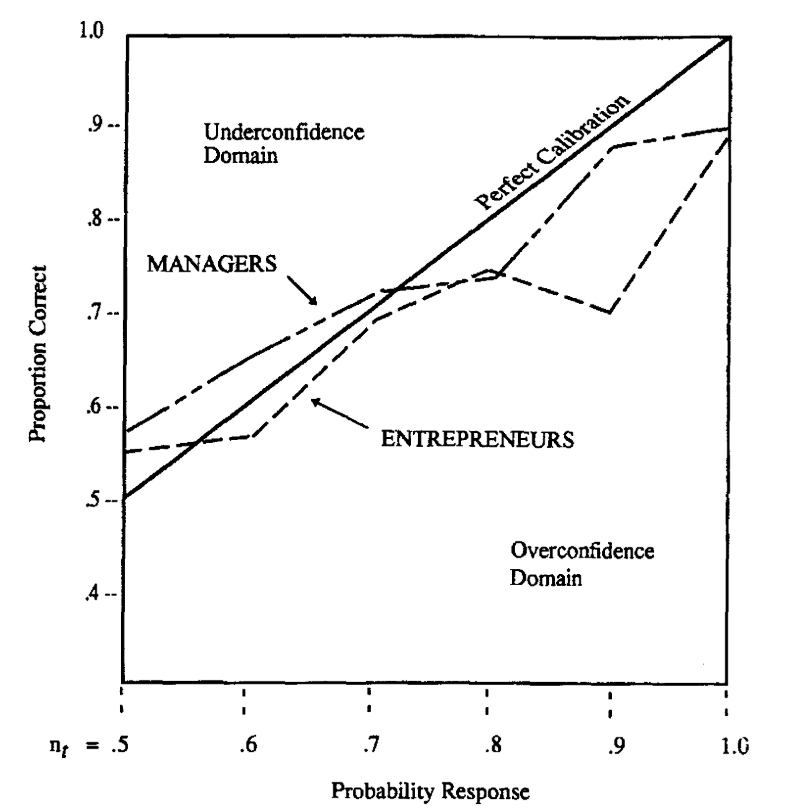
To measure representativeness, Busenitz and Barney provided subjects with two separate scenarios representing various types of real-life strategic decisions. Each scenario consisted of two alternatives, one of which subjects chose as their preferred alternative. Scenario 1 involved the purchase of a major piece of equipment, whereas scenario 2 depicted an automation update decision. After deciding on their preferred alternative, subjects described their reasoning behind each decision. Coders then analyzed the responses to determine the extent to which heuristic-type reasoning was used by subjects in determining their preferred alternative. A code of “1” was assigned to responses that contained no mention of statistical reasoning, relying instead on subjective opinions or simple rules of thumb. Examples of this form of reasoning include reference to personal experience or simple decision rules like “buy American.” A code of “0” was assigned to responses containing some form of statistical reasoning, including references to variability or sample size. Finally, the results for both scenarios were summed to create a single three-category variable (0-2), with a “0” indicating that the subject used statistical reasoning across both problems, and a “2” indicating that only heuristic reasoning was used.

The table below presents results for logistic regression analysis, where, for those of you familiar with this type of analysis, the dependent variable represents entrepreneur versus manager (coded “2” if the former and “1” if the latter). Given this coding of the model’s dependent variable as well as the coding for the overconfidence and representative measures, we expect coefficients associated with these measures to be positive and statistically significant, which, as we see, they are.

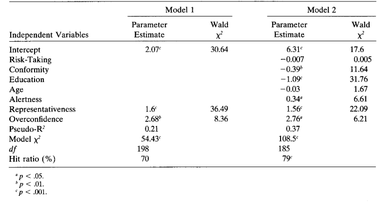
Model 1 includes solely the representativeness and overconfidence measures as explanatory variables, whereas Model 2 includes a host of control variables measuring a subject’s proclivity for risk-taking and conformity, degree of alertness, as well as level of education and age. In both models, the coefficients for representativeness and overconfidence are indeed positive and statistically significant, and these two measures by themselves correctly distinguish entrepreneurs from managers more than 70% of the time (as indicated by the Hit Ratio statistic). These results suggest that Representativeness and Overconfidence Biases manifest themselves more in the strategic decision-making behavior of entrepreneurs than managers.

It should come as no surprise that differences such as these would not arise with Homo economicus entrepreneurs and managers since neither group would be susceptible to Representativeness and Overconfidence Biases to begin with.

Beneficial Heuristics Too

The implication of the two heuristics discussed in Chapter 1—the Affect and Availability Heuristics—is that heuristics generally lead to misjudgments on the part of Homo sapiens. As Gigerenzer and Gaissmaier (2011) point out though, this is not always the case. The use of heuristics can sometimes lead to more preferable outcomes than those determined by statistical analyses or more complex strategies.

For example, consider the Hiatus Heuristic, where a customer who has not purchased anything from a business within a certain number of months (the hiatus) is classified as inactive. In their study of an apparel retailer, an airline, and an online CD retailer—whose Hiatus Heuristics were nine, nine, and six months, respectively—researchers Wübben and Wangenheim (2008) compared this heuristic to a statistical analysis of 40 weeks of data from each company.^[50] The heuristic resulted in a correct classification of an inactive customer if the customer did not make a purchase during the 40-week period of analysis (which is one month longer than the nine-month hiatus period for the apparel retailer and airline, and four months longer than the CD retailer’s six-month hiatus period).^[51]

For the apparel retailer, the Hiatus Heuristic correctly classified 83% of customers, whereas the statistical model classified only 75% correctly. For the airline, the Hiatus Heuristic correctly classified 77% of the customers versus 74% for the statistical model, and for the CD retailer, the two approaches each correctly classified 77% of the customers.

Another beneficial heuristic identified by Gigerenzer and Gaissmaier (2011) is known as the “Recognition Heuristic,” whereby if an individual first determines a criterion upon which to judge the value of some alternative, say alternative A, and alternative A is later recognized among the other alternatives, then the individual infers that alternative A has the higher value associated with that criterion.^[52] For example, in predicting federal and state election outcomes in Germany, forecasts based upon surveys of how well voters recognized the candidates’ names performed almost as well as interviews with voters about their actual voting intentions (Gaissmaier and Marewski, 2010). Similarly, in three studies conducted by Ortmann et al. (2008) designed to predict the stock market, recognition-based portfolios (i.e., stock portfolios comprised of the most-recognized companies) on average outperformed managed funds such as the Fidelity Growth Fund, the market (Dow or DAX), chance portfolios, and stock experts.

The One-Clever-Clue Heuristic is used in a myriad of circumstances. For example, Snook et al. (2005) study the use of geographic profiling to predict where a serial criminal is most likely to live given the locations of a series of crimes. Typically, geographical profiling utilizes a sophisticated statistical software program to calculate probability distributions across possible locations. The authors tested a special case of the One-Clever-Clue Heuristic, which they named the Circle Heuristic. The Circle Heuristic predicts the criminal’s most likely location simply as the center of a circle drawn through the two most distant crime locations. The heuristic thus relies on one cue only: the largest distance. In a comparison with 10 other profiling distributions, the Circle Heuristic predicted the locations best. Nevertheless, the authors found that complex profiling strategies became more accurate as the number of crime locations was no less than nine.

As Gigerenzer and Gaissmaier (2011) point out, the Take-The-Best Heuristic is similar to the One-Clever-Clue Heuristic, except that clues are retrieved from the individual’s memory. Perhaps the most famous example of how the Take-The-Best Heuristic has been used effectively is Green and Mehr’s (1997) study of how patients are assigned to the coronary care unit (CCU) at a Michigan hospital. When a patient arrives at any hospital with severe chest pain, emergency physicians have to decide quickly whether the patient suffers from acute heart disease and should therefore be assigned to the CCU. Historically, at the Michigan hospital in question doctors preferred to err on what they considered to be the safe side by sending 90% of the patients to the CCU, although only about 25% of these patients typically had critical symptoms. This created overcrowding in the CCU and a concomitant decrease in quality of care.

Green and Mehr (1997) tested two approaches. One was the use of a logistic regression equation known as the Heart Disease Predictive Instrument (HDPI). The other was a simple decision tree depicted in the figure below. Accordingly, if the answer to the question of whether an ST segment has changed is “yes,” then the patient is immediately sent to the CCU. If “no,” and the patient’s chief complaint is chest pain, his condition is assessed for one of a few other factors. If a factor is present, the patient is then sent to the CCU. If the patient’s ST segment has not changed and he either does not complain of chest pain or another factor is not present, then the patient is provided with a regular nursing bed.

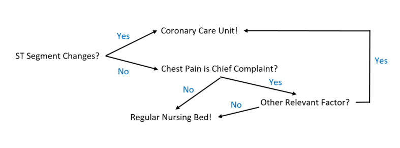
To use the HDPI, doctors review a complex chart consisting of approximately 50 different possible symptoms and enter what they consider to be the probabilities of relevant symptoms into a pocket calculator. Green and Mehr (1997) found that the decision tree was more accurate in predicting actual heart attacks than the HDPI—the use of the decision tree sent fewer patients who suffered from a heart attack to a regular bed and also nearly halved physicians’ high false-alarm rates (i.e., the sending of patients to the CCU when they instead should have been sent to a regular bed). Because the decision tree was a transparent and easy-to-memorize heuristic, the hospital’s physicians preferred its use.

As this brief discussion indicates, there are a plethora of ways in which Homo sapiens actually outsmart Homo economicus through the use of heuristics. Indeed, Gigerenzer and Gaissmaier (2011) report on a study showing that a simple physician’s bedside exam can outperform the use of a magnetic resonance imaging (MRI) exam in the diagnosis of a brainstem or cerebellar stroke, and another showing how the simple 1/N Rule, where resources (e.g., time or money) are allocated equally over N different alternatives, can outperform more sophisticated optimization models. These are specific examples of Trade-Off Heuristics. The point is that the simpler mind of Homo sapiens does not always put her at a disadvantage relative to the more complex mind of her Homo economicus muse.

If You Give a Grocery Shopper a Muffin

Gilbert et al. (2002) ran a field experiment to test for the presence of Projection Bias among roughly 100 grocery store shoppers. The shoppers were stopped in the parking lot on their way into the store and asked to participate in a Taste Test and Survey Study. Participating shoppers began by making a list of the items they planned to purchase that day in the store (shoppers who had already created their own lists were politely informed that they were ineligible to participate). Participants were randomly chosen to either receive their lists back before entering the store (henceforth known as “listful” shoppers), or not receive their lists back (“listless” shoppers). Next, participants were assigned to one of two groups. One group was given muffins to eat before entering the store (henceforth known as “sated” shoppers). The other group was asked to return after having completed their shopping to pick up their muffins (“hungry” shoppers). On average, sated shoppers both listful and listless later self-reported themselves as feeling less hungry after having completed their shopping trip than listless and listful hungry shoppers.

After shopping, each shopper’s receipt was collected. The authors found that, on average, listless sated shoppers made significantly fewer unplanned purchases than listless hungry shoppers. In specific, over 50% of the purchases made by the listless hungry shoppers were unplanned, versus only 34% of purchases made by listless sated shoppers. The difference between listful sated and listful hungry shoppers was not statistically significant. The authors concluded that when we are hungry, food is attractive. When unconstrained by a pre-made shopping list, the items we pass in the grocery store are thus more likely to be evaluated based upon how they would satisfy our current, rather than future, hunger.^[53] As such, listless sated shoppers effectively de-contaminate their hedonic mental representations of consuming their food purchases in the future by shopping with less hunger in the present (i.e., they are less likely to suffer from Projection Bias of their future food consumption needs). Shopping with the intent of accurately satiating future hunger is, after all, the point of one’s weekly grocery trips!

Catalog Sales and Projection Bias

It is no surprise that in the rational-choice model of Homo economicus, individuals accurately predict how their tastes for different goods and services change over time. It should likewise come as no surprise that no such accuracy attends the predictions made by Homo sapiens. Loewenstein et al. (2003) hypothesized that Homo sapiens exhibit a systematic Projection Bias when it comes to accounting for changes in their tastes. While they tend to understand the direction in which their tastes change (e.g., that eating the same foods for dinner over and over diminishes one’s appetite for those foods), Homo sapiens systematically underestimate the magnitudes of these taste changes.

In a nifty field experiment, Conlin et al. (2007) set out to test this hypothesis by analyzing catalog orders for weather-related clothing items and sports equipment. The authors find evidence of Projection Bias with respect to the weather, in particular, that Homo sapiens are overinfluenced by weather conditions at the time they make decisions on what to order. Specifically, if the weather on the day he places an order from the catalog would make the item seem more valuable if used on that day, then he is more prone to order the item. For example, with cold-weather items (i.e., items that are more valuable in colder temperatures), Conlin et al.’s dual hypotheses are that the likelihood of returning the item is (1) declining in the order-date’s temperature (order-date hypothesis), and (2) increasing in the return-date’s temperature (return-date hypothesis). In other words, a lower order-date temperature or a higher return-date temperature is associated with a higher probability of returning the item. As a consequence of these temperature differentials, an individual’s likelihood of returning the item after having received it should increase, which would demonstrate a Projection Bias on both the day the item was ordered and the day it was received.

To test these hypotheses, the authors obtained sales data from a large outdoor-apparel company. The company provided usable, detailed information on over 2 million orders of weather-related items, including the zip code of the buyer, the order date, and whether the item was ultimately returned. Specifically, the company provided information about each item ordered, its order date, the date the item was shipped, whether the item was returned, and, if so, the date on which the company restocked the item. In addition, the company provided information on the five-digit zip code associated with the billing address, whether the shipping address was the same as the billing address, the price of the item purchased, whether the order was placed over the Internet, by phone, or through the mail, and whether the buyer used a credit card to purchase the item. The company also provided information that enabled the authors to construct a two-day window during which the buyer was most likely to have received the item. The authors then merged this data with daily weather information for each zip code in the US.

Conlin et al. ultimately find support for their order-date hypothesis—a decline in the order-date’s temperature of 30°F is associated with an increase in the return rate of roughly 4%. However, they do not find support for the return-date hypothesis. Their specific econometric results are presented in the table below:

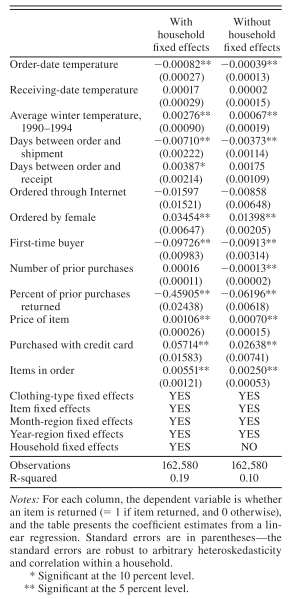
As the table indicates, the coefficient estimate for order-day temperature, with and without “household fixed effects,” is negative and statistically significant.^[54] In other words, a lower order-date temperature is indeed associated with a higher probability that the item will later be returned (i.e. evidence of Order-Date Projection Bias). To the contrary, the authors do not find strong support for the return-date hypothesis. While the coefficient estimate on receiving-date temperature is positive and larger when household fixed effects are controlled for, the coefficients are not statistically significant.

Poor Homo sapiens. I don’t know about you, but I find returning items I’ve previously purchased to be a hassle; a hassle Homo economicus never experiences.

Student Procrastination

Caplan and Gilbert (2008) define two different types of student procrastination—“late-starting” and “back-loading.” As their names suggest, late-starting procrastination occurs when a student gets started on a homework assignment closer to the assignment’s due date, and back-loading procrastination occurs when a student (who may have started early on an assignment) waits until later (closer to its due date) to finish the assignment. Assessing grades on a series of homework assignments completed by students in an intermediate microeconomics course, the authors found that both late-starting and back-loading procrastination reduce the typical student’s score on any given homework assignment.

Using data compiled by the course’s web-based course-management tool, Caplan and Gilbert (2008) were able to define late-starting according to the difference (in days) between an assignment’s grading deadline and when the student first accessed the assignment online to answer one of its questions.^[55] They defined back-loading according to skewness in the distribution of a student’s time differences (in minutes) between an assignment’s grading deadline and when a student first accessed each of the assignment’s questions. The greater the extent of positive skewness in a student’s time distribution, the more the student back-loaded the assignment.

The authors found that for each day a student late-started an assignment, his score fell by slightly less than 3%. Back-loading resulted in a slightly less than 2% reduction in the assignment’s grade per unit of skewness. The results controlled for whether a student attempted an assignment’s practice problems beforehand, the student’s grade point average (GPA), total credits enrolled for the semester, gender, total number of hours worked per week at a wage-paying job, number of children under the age of 18 years living in the household, and which third of the semester each assignment was given. Caplan and Gilbert (2008) conclude that procrastinators, both late-starting and back-loading, tend to perform worse on graded assignments than their non-dillydallying counterparts.

Stopping Procrastination Dead With Deadlines

In an attempt to better understand the propensity of Homo sapiens to control their procrastination through self-imposed deadlines (as a Commitment Mechanism) and whether this type of “binding behavior” can improve task performance, Ariely and Wertenbroch (2002) involved approximately 100 executive-education students at the Massachusetts Institute of Technology (MIT) in a semester-long field experiment.^[56] Fifty-one students were randomly assigned to a “free-choice” treatment group where they were free to set their own deadlines for three short papers throughout the semester, and 48 students were assigned to a “no-choice” control group where they were assigned fixed, evenly spaced deadlines for the three papers.^[57] The authors found that, on average, the deadlines set by the free-choice students were roughly 33, 20, and 10 days before the end of the course for papers 1, 2, and 3, respectively.

Overall, less than 30% of the deadlines were set by free-choice students for the final week of class (calculated as roughly 45 out of a total of 153 papers (3 papers x 51 students in the group)). The majority of deadlines were set prior to the final lecture (27% of the free-choice students chose to submit all three papers on the final day of class). The results suggest that students are willing to self-impose deadlines to overcome procrastination even when the deadlines are costly (in terms of a grade penalty for missing a deadline).

Ariely and Wertenbroch (2002) also compared grades across the free-choice and no-choice groups to see if flexibility in setting deadlines enabled members of the former group to attain higher grades than members of the latter group. The authors found that, on average, grades were higher in the no-choice group, suggesting that the free-choice students suffered from self-control problems, and although they used the deadlines to help overcome these problems, they did not set the deadlines optimally. The greater flexibility afforded the free-choice students ultimately led to worse performance.

The moral of Ariely and Wertenbroch’s story? There is a potential tradeoff for Homo sapiens between stopping procrastination dead in its tracks and one’s overall performance of the task at hand.

Testing the Small-Area Hypothesis

A question loosely related to why Homo sapiens procrastinate is, what factors influence an individual’s motivation to bring goals to completion? As Koo and Fishbach (2012) point out, previous research suggests that the closer people are to reaching a goal, the more resources they are willing to invest to reach it. For example, in the context of reward programs, consumers are more likely to make a purchase, and make it sooner, if they are only a few purchases away from receiving the reward. Homo sapiens in general prefer actions that appear more impactful and thus increase their perceived pace of progress. Drawing from this logic, Koo and Fishbach set out to test the Small-Area Hypothesis, which proposes that how people monitor their progress toward goal completion influences their motivation.^[58] In particular, the authors distinguish between the framing of progress in terms of completed actions versus remaining actions to complete a goal. They hypothesize that when people start pursuing a goal, a focus on accumulated progress (e.g., 20% completed) is more motivating than a focus on remaining progress (e.g., 80% remaining). Then, toward the end of their pursuit, a focus on remaining progress (e.g., 20% remaining) is more motivating than a focus on completed progress (e.g., 80% completed). In other words, directing attention to small areas increases motivation because the marginal impact of each action toward goal achievement then appears relatively larger.

To test this hypothesis, Koo and Fishbach conducted a field experiment in a sushi restaurant that offered a buffet lunch menu located in a major metropolitan area in South Korea. For four months, they ran a reward program in the format of “buy 10 meals, get one free.” The program manipulated customers’ attention to accumulated versus remaining progress by providing them with a frequent buyer card on which they either received a stamp for each meal purchase (i.e., focus on accumulated progress) or had a slot removed for each meal purchase (i.e., focus on remaining actions needed). Over the four-month period, the researchers issued 907 reward cards corresponding to 907 participants, though some customers may have redeemed one card and then received another, leading them to participate in the study more than once. The restaurant served a lunch sushi buffet for 20,000 won (US $18) per person. Koo and Fishbach offered the reward program solely for lunch buffet meals.

Participants in the field experiment received a frequent-buyer card similar to the ones displayed in the figure below. Participants were randomly assigned to one of two conditions. In the accumulated-progress condition, participants received a card to which a sushi-shaped stamp was added from left to right for each purchase (Card A in the figure). Thus, participants in this condition were provoked to direct their visual attention to the number of completed stamps. The text on the card indicated that customers would get a sushi stamp per every lunch meal and would be eligible for a free lunch meal once they received 10 stamps. In the remaining-progress condition, participants received a card with 10 printed sushi pictures already included (Card B in the figure). A punch was used to remove one picture from left to right for each purchase. In this condition, the participants were provoked to direct their visual attention to the number of remaining slots. The instructions on the card stated that a slot would be removed per every lunch meal purchased and that customers would be eligible for a free lunch meal after all 10 sushi pictures were removed.

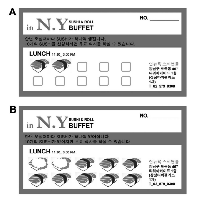
To assess a participant’s initial progress, the authors recorded the number of purchases made at the time each reward card was issued. Because a single customer often paid for several lunches at the same time (covering the cost of her friends’ meals), Koo and Fishbach were able to obtain natural variations in the level of progress customers made on their first visit. Overall, participants who attained a higher level of progress were more likely to use the card again (a result nevertheless driven by those who received a card with 10 printed sushi pictures already included). As the authors point out, this result reflects a Goal-Gradient Effect—those who made more purchases on the first visit were closer to the reward of the free meal and thus more likely to revisit the restaurant for a second time. Participants were more likely to revisit with the card highlighting remaining (vs. accumulated) purchases, possibly because attention to accumulated purchases encourages “resting on one’s laurels.”

Most importantly, these results indicate that high-progress participants (i.e., participants who purchased more meals initially) were more likely to revisit the restaurant if their card emphasized remaining purchases. Conversely, low-progress participants were more likely to revisit the restaurant with the card emphasizing accumulated purchases. As the authors state, this pattern supports the Small-Area Hypothesis—the higher the initial progress, the smaller the remaining-purchases area; and the lower the initial progress, the smaller the accumulated-purchases area.

Koo and Fishbach also measured how quickly participants revisited the restaurant by analyzing the number of days between the card’s issuance and the participant’s second visit to the restaurant. High-progress participants revisited the restaurant more quickly (i.e., within a shorter interval of days), a result driven mainly by those participants with cards emphasizing remaining purchases. Conversely, low-progress participants revisited the restaurant sooner if their card emphasized accumulated purchases. Hence, the Small-Area Hypothesis is again supported, this time regarding the amount of time elapsing between a participant’s first and second visits to the restaurant.

The take-home message from this experiment is clear. If you are in the position of having to nudge yourself or someone else to accomplish a goal, you are more likely to attain that goal if you focus your persuasive messaging on the smaller of the two areas: the progress already made toward attaining the goal vs. the effort remaining to reach it. It is interesting to note that Homo economicus‘ behavior would not satisfy this hypothesis. It matters not which type of card is initially issued.

Excessive Planning

Setting personal goals and constructing respective plans to achieve them is a time-honored tradition of the Homo sapiens experience, so much so that a multitude of luminous thinkers have weighed in with memorable witticisms. A goal without a plan is just a wish (Antoine de Saint-Exupéry); By failing to prepare you are preparing to fail (Benjamin Franklin); If you don’t know where you are going, you’ll end up someplace else (Yogi Berra); and my three favorites, Plans are of little importance, but planning is essential (Winston Churchill); Always plan ahead. It wasn’t raining when Noah built the ark (Richard Cushing); and, Good fortune is what happens when opportunity meets with planning (Thomas Edison).^[59] One gets the distinct impression that the more planning the better.

Kirschenbaum et al. (1981) set out to test this impression in the context of a field experiment conducted with over 100 students at the University of Rochester during the spring semester of 1979. The students’ goals were to leverage more structured and elaborate planning to enrich their studying time and ultimately improve their grades. The authors’ goals were to test whether plans varying in specificity (i.e., detailed plans specifying a daily schedule (“daily plans”) or looser plans outlining a monthly schedule (“monthly plans”)), have differential impacts on the students’ self-regulated study behaviors. The authors hypothesized that (1) students following daily plans would experience both greater process gains (i.e., with respect to developing more effective study habits) and performance gains (i.e., higher grades) than those following monthly plans; and (2) irrespective of whether they were following daily or monthly plans, students assigned to participate in an 11-session Study Improvement Program (SIP) would experience greater process gains than students in a control group that neither participated in the SIP nor devised plans for improving their studying effectiveness.

Kirschenbaum et al. recruited students with varying academic majors, half of whom were first-year undergraduates on academic probation or close to being on probation, who agreed to participate in the SIP. Students were first divided into “low-grade” and “high-grade” groups, the low-grade group consisting of students with cumulative grade point averages (GPAs) of 2.1 or less and the high-grade group with GPAs greater than 2.1. Roughly half of the low- and high-grade group members were then randomly assigned to respective control groups. The other halves were randomly assigned to one of six different treatment groups: daily plans-low grades, daily plans-high grades, monthly plans-low grades, monthly plans-high grades, no plans-low grades, and no plans-high grades.^[60]

Students assigned to the daily and monthly plan groups used their course syllabi and textbooks to complete their plans (flow charts), which were then reviewed by other participants in the group and group leaders. The plans specified tasks to be accomplished, where and when they were to be worked on, the criterion of accomplishment, the self-administered reward to be earned, and where and when the reward was to be allocated. Daily-plan students completed highly specific plans in which they indicated study behaviors (e.g., activities, criteria, rewards) pertaining to each day (four days were planned on each flow chart). In contrast, monthly-plan students developed less-specific plans indicating larger chunks of activities that spanned one month’s work on each flow chart, including a reward to be self-administered at the end of the month if the criterion level of accomplishment was achieved. Both groups were instructed to continue creating new plans when their flow charts became outdated (i.e., once a month for monthly plans and once every four days for daily plans). Daily-plan students also graphed their study time every day, while monthly-plan students graphed total study time each month. All participants self-monitored their study time on a daily basis.

Over the course of the ensuing semester, Kirschenbaum et al. found that monthly-plan students self-monitored more study hours and more “effective” (i.e., undistracted) study hours, and indicated less of a tendency to procrastinate, than did daily- and no-plan students. Monthly-plan students also maintained a relatively high rate of studying throughout the semester, whereas both daily- and no-plan students decelerated their study hours from the first to the second five-week period of the semester. While the authors found that within their cohorts both low-grade and high-grade students who participated in the SIP improved their GPAs relative to their respective control groups (i.e., low-grade SIP student GPAs improved relative to low-grade control group student GPAs and similarly for the high-grade SIP and control groups). No other statistically significant effects were found for student performance. High-grade students with daily and monthly plans did not perform better than high-grade students without plans, and similarly for low-grade students with and without plans.

Kirschenbaum et al. conclude that daily planning may have inhibited effective self-regulation by overburdening students with the task of planning for each day or by causing negative reactions in students who failed to meet their daily criteria for positive evaluation. In contrast, by writing out a proposed schedule for a longer period of time, monthly-plan students were able to increase their perception of control or choice. Either way, these results suggest that wise though it may be, students should be wary of the sage advice about planning far in advance.

Keep Your Options Open?

Remember the old saying, Jack of all trades, master of none? It has historically (and pejoratively) distinguished someone who has developed relatively low-level competencies in a number of different occupations from one who has mastered the skills required of a single occupation. Each of us likely knows someone who has excelled in (i.e., mastered) their career at the expense of developing their skills in other facets of life, and someone who has dabbled in (i.e., jacked) different trades but never quite built a career in any one of them. Another example is someone who lacks hesitation when it comes to making decisions—they tend to “jump right in”—versus someone who likes to keep their options open, and thus typically takes more time in making up their mind. Homo sapiens can indeed be fickle this way.

In an interesting set of experiments, Shin and Ariely (2004) investigate the extent to which Homo sapiens’ penchant for keeping our options open leads to making inefficient choices. The authors ask whether the threat of future unavailability makes currently less-desirable options seem more appealing and whether this causes Homo sapiens to overinvest in these less-desirable options. In other words, do doors that threaten to close appear more attractive than doors that remain open? And if so, will individuals overinvest just to keep them open? As Shin and Ariely point out, we would expect Homo economicus to value an option (having the ability to make a choice) based solely upon the expected utility of the outcomes the option provides. To the contrary, we would expect Homo sapiens to be swayed by a preference for flexibility and by loss aversion, causing an option’s subjective value to exceed its expected value.

Shin and Ariely’s experiments all followed the same basic procedure. Participants interact with a computer game consisting of three different doors opening to three different rooms. One door is red, another blue, and the third green. By clicking with the mouse on one of the doors (i.e., by door-clicking), a participant opens the door and enters the room. Once in the room, the participant can begin clicking repeatedly in the room (i.e., room-clicking) to obtain points randomly drawn from a given distribution of points, or, after any number of room-clicks within one room, door-click another door (for no points on that click) to begin clicking in the new room for points randomly drawn from a different (albeit mean-preserving) distribution of points. The expected value and other moments of each distribution are unknown to the participants. Note that charging a participant a click for switching rooms creates a switching cost. The total number of clicks is prominently displayed on the computer screen, in terms of how many clicks have been used and how many remain until the end of the game.

Participants were initially given a “click budget” to use on door- and room-clicks at their discretion. Once participants used up all their clicks the game ended and they were paid the sum of their room-click payoffs. The main goal of the experiment was to measure the relationship between the actions of a participant and door availability (i.e., “option availability”), which varies on two levels: “constant availability” or “decreased availability.” Under constant availability, all three rooms remain viable options throughout the experiment, irrespective of a participant’s actions. Under decreased availability, door availability depends upon the actions of the participant. Each time the participant clicks on a door or within a room, the doors of the other two rooms decrease in size by 1/15th of their original width. A single door-click on a shrinking door re-sizes it to its original size and the process continues. If a door’s size reaches zero it is eliminated for the remainder of the game. Poof!

Shin and Ariely’s first experiment was designed to test the hypothesis that as doors shrink in the decreased-availability treatment, participants will invest in keeping their options open (i.e., spending a click to reverse a door’s shrinkage). For this experiment, the expected value of a room-click (in any room) was 3 cents; however, the doors’ point distributions were (1) Normal with a variance 2.25 cents and min/max 0/7 cents, (2) Normal with a variance 0.64 and min/max 1/5, and (3) Chi-Square with a variance 10 and min/max -2/10 for doors 1 – 3, respectively. Each participant was given a budget of 100 clicks. Over 150 students participated.

Shin and Ariely found that door switching was indeed significantly more likely to occur under decreased as opposed to constant availability. The authors also found that, overall, there was a decreased tendency among participants to switch rooms later in the game. However, more switching still occurred in the decreased-availability treatment. The authors point out that as click numbers increase, participants are gaining more experience, can better estimate the point distributions, and thus should have less of a need to explore other rooms (i.e., options). Further, the expected value of exploring other options is reduced with click number because the time horizon during which this constantly improving information can be put to use is being reduced.

It turns out that because of switching costs, picking a room and remaining there for the duration of the experiment is the optimal (rational) strategy in terms of earning the highest expected payout from the experiment (yes, this would be Homo economicus’ strategy). Indeed, Shin and Ariely calculate that across both the constant- and decreased-availability treatments participants surrendered 11% of their payouts as a consequence of switching rooms (the average participant switched rooms 12 times during the course of the experiment).

Shin and Ariely’s second experiment manipulated participants’ knowledge about the point distributions for the various rooms, the hypothesis being that providing more information should substantially reduce the difference in switching between the constant- and decreased-availability treatments. On the other hand, if the information provided does not reduce this difference, then the difference is driven by a preference for flexibility and loss aversion rather than a paucity of information. The authors found evidence for the latter—Homo sapiens exhibit an inherent tendency to keep their options open—borne of a preference for flexibility in decision making or by loss aversion, even when doing so is costly.

Anticipated Versus Unanticipated Income

In a series of laboratory experiments, Arkes et al. (1994) tested whether Homo sapiens tend to spend (as opposed to save) unanticipated income (affectionately known as windfall gains) to a greater extent than anticipated gains (e.g., from owned assets). This is a non-issue for Homo economicus, who would never succumb to the temptation of spending more lavishly from unanticipated income. One experiment (Experiment 1) was designed to test whether students receiving unanticipated income would be more likely to risk that income on a simple lottery. The other experiment (Experiment 2) tested whether students receiving unanticipated income were more likely to spend the income on a consumer good. In each experiment, one randomly chosen group of students (the control group) arrived at the experiment anticipating some payment while the other group (the treatment group) was surprised by being given a payment upon arrival.

Students in both the treatment and control groups were informed between one and five days ahead of the experiment about the experiment’s time and location. Students in the control group were also provided the following information:

Although it wasn’t mentioned on the sign-up sheet for participating in the experiment, we want you to know that you will be paid for being in this experiment. We usually pay all our subjects $3.00 for participating. You will be paid when you get there. I thought you should know that. Also, I’d like to ask you not to mention to anyone that you’re being paid. The reason for this is that not all psychology experiments pay the participants, so it’s better if no one knows one way or the other.

This additional information effectively distinguishes anticipated income (obtained by members of the control group) and unanticipated income (eventually obtained by members of the treatment group). Members of the treatment group unexpectedly received the $3 just prior to the start of the experiment. Unlike members of the control group, treatment-group members were not provided with any information prior to the experiment.

After receipt of the $3 the control- and treatment-group students participating in Experiment 1 were presented with the following gamble:

You can bet as much of your $3 on the roll of a pair of dice, from 25₵ to the entire $3. If you roll a number seven or greater, you win. If you roll a number less than seven, you lose. For example, if you bet $1 and you roll a number seven or greater, I will pay you $1. If you roll a number less than seven, you will pay me $1. You can roll the dice only once. Do you understand? How much do you want to bet?

Students in the control group wagered an average of $1 on the gamble, while those in the treatment group wagered a statistically different average of $2.16. In other words, those students experiencing a windfall gain of unanticipated income wagered more than double the amount of income on the gamble than students whose gain in income was anticipated.

Control- and treatment-group students participating in Experiment 2 were distinguished in the same manner as in Experiment 1. However, in this case, the students were paid $5 rather than $3, and rather than subsequently facing a gamble, the students were sent to a basketball game. After the game, the amount of the $5 each student spent on concessions at the game was tallied.

Similar to the results from Experiment 1, students in the control group spent an average of just under 40₵ at the game while those in the treatment group spent a statistically different average of 90₵. This is yet another indication that Homo sapiens tend to be more spendthrift with windfall gains!

Optimistic Overconfidence in the Stock Market

As Barber and Odean (2001) point out, theoretical models of investor behavior predict excessive trading in the stock market by overconfident investors. Likewise, psychological research demonstrates that in areas such as personal finance, men are more overconfident than women (c.f. Karabenick and Addy, 1979). Together, these two theories predict that men will trade more excessively than women, a prediction the authors test by partitioning investors according to gender. Using account data for over 35,000 households from a large discount brokerage, they analyze the common stock investments of men and women over the course of six years, from 1991 through 1997. The authors find that men trade 45% more of their portfolios than women and that trading reduces men’s net returns by 2.65 percentage points per year (relative to what their net returns would have been had they not traded) as opposed to a 1.72 percentage-point reduction in net returns for women traders.

Barber and Odean (2001) find that, across all households in the sample, men’s average monthly turnover of stocks in their portfolio (technically defined as where = shares sold, = beginning-of-month price per share, and = total beginning-of-month market value of the owner’s portfolio) was roughly 2% greater than the average woman’s. This average difference in turnover rate between men and women was larger than that for the subsample of married households and lower than that for single-headed households. Across all households, women traders earn net monthly returns (what Barber and Odean call own-benchmark monthly abnormal net returns) that are 0.143% lower than those earned by the portfolio they held at the beginning of the year, while men traders earn net monthly returns that are 0.221% lower than those earned by the portfolio they held at the beginning of the year. Both shortfalls are statistically significant at the 99% confidence level, as is their difference of 0.078%. As with the stock turnover rates, the differences in net monthly returns between men and women traders are lower among married households and higher among single-headed households.

Bottom line for Homo sapiens? Not only are men overconfident in their investing acumen relative to women, but they also suffer larger losses in their investment portfolios than they otherwise would had they not been so confident in their investing abilities.^[61]

The Equity Premium Puzzle

As pointed out by Benartzi and Thaler (1995), historically there has been an enormous discrepancy between the returns on equity (e.g., stocks) and fixed-income securities (e.g., treasury bills and bonds). Since 1926, the annual real return on stocks has been roughly 7% while, for treasury bills, the return has been less than 1%. In an early attempt to explain the extent of this “equity premium,” Mehra and Prescott (1985) found that plausible levels of investor risk aversion were an unlikely culprit, which, in turn, signaled the need for an explanation grounded in a framework other than that offered by the rational choice model of Homo economicus. What makes it so puzzling is not so much that the premium exists. Rather, given the premium exists, why would investors ever choose to hold securities?

Benartzi and Thaler offer an explanation for this puzzle that is firmly rooted in Prospect Theory. Investors are by nature loss averse, and long-term investors evaluate their portfolios frequently. Together, these two traits of Homo sapiens investors lead to what the authors call myopic loss aversion. In conjunction with being loss averse, the more often he evaluates his portfolio (i.e., the shorter his evaluative horizon), the less attractive an investor finds a high mean, high-risk investment such as stocks. By being loss averse, the investor effectively overreacts to the downside risk (i.e., when his stocks fall in value) and therefore over-invests in treasury bills or bonds.

The authors demonstrate how myopic loss aversion among investors can explain the equity premium puzzle by answering the question, “If investors exhibit myopic loss aversion, how often would they have to evaluate their investment portfolios in order to explain the equity puzzle” (page 81)? To answer this question, Benartzi and Thaler draw samples from the historical (1926-1990) monthly returns on stocks, bonds, and treasury bills provided by the Center for Research in Security Prices (CRSP). Using this data, they can simulate prospective utility levels associated with portfolios holding purely stocks and purely bonds for evaluation periods starting at one month and increasing one month at a time. The authors find that the evaluation period at which stocks and bonds are equally attractive, i.e., where the common portfolio consisting of 50% stocks and 50% bonds is optimally held, occurs at roughly 13 months. In other words, the common portfolio is most likely to occur when the representative investor evaluates stock and bond returns roughly once per year.

The moral of this story is striking. Because stock returns have historically outperformed bond returns, there is no reason to believe that a pure stock portfolio (or at least a portfolio heavily weighted in stocks) should not continue to outperform a portfolio more heavily weighted in bonds. Therefore, if you are a Homo sapiens prone to suffer from myopic loss aversion, it is best to invest in a stock portfolio at the outset, and then avoid evaluating your returns for as many years as you can. Yes, this is a case where procrastination (in reviewing your stock portfolio) actually pays off!

If constraining yourself to this extent places too heavy a burden on your curiosity, then at the very least consider practicing what Galai and Sade (2006) and Karlsson et al. (2009) have coined the Ostrich Effect. This effect occurs when an investor evaluates his returns more often after a rise in the stock market (i.e., after receiving good news) than after receiving bad news about a fall in the market. By practicing the Ostrich Effect an investor helps to offset the inherent, negative impacts of myopic loss aversion.

Endowment Effects Among Experienced Versus Inexperienced Traders

In Chapter 6, a simple laboratory experiment was proposed to test for an Endowment Effect in a constructed market setting. We surmised that in a market characterized by a relatively strong endowment effect exhibited by the sellers, one would expect most sellers’ WTA values to exceed buyers’ WTP values, resulting in few sales ultimately being consummated. In other words, to the extent that Homo sapiens sellers betray an Endowment Effect, we would not expect them to behave like their dispassionate Homo economicus counterparts, who, by virtue of their immunity to such an effect, would likely consummate more sales in the market and thereby generate larger gains from trade.

Experimenting in a constructed market setting has its advantages, foremost among them the ability of the experimenter to mitigate potential confounding factors correlated with any given real-world context. However, as List (2004) demonstrates, when it comes to testing for an Endowment Effect among sellers of an everyday consumable good, a well-functioning, real-world marketplace provides an ideal setting for a field experiment. In such a marketplace (which in List’s case is a sports card trader’s show), List can distinguish experienced from inexperienced sellers and thus measure the divergence in the strength of the Endowment Effect among these two seller types. In his experiment, List’s “everyday consumable goods” are candy bars and coffee mugs. He finds that inexperienced sellers exhibit a relatively strong Endowment Effect. Experienced sellers behave more like Homo economicus; they are capable of eschewing the endowment urge.

List designed two versions of his experiment—one in which the market mimics a typical private market where buyers and sellers interact in an uncoordinated setting (Experiment 1), the other in which a collective-choice mechanism guides the sellers’ individual decisions toward a coordinated outcome (Experiment 2).

In Experiment 1, each subject was randomly assigned to one of four treatments. The treatments differ by type of endowment. Subjects in treatment  are initially endowed with one coffee mug, subjects in treatment  one candy bar, subjects in treatment  one mug and one candy bar, and subjects in treatment  neither a mug nor a candy bar. The coffee mug retailed for just under $6 at the University of Arizona bookstore. The candy bar was an extra-large, fine Swiss chocolate bar that also sold for roughly $6.00. Fundamental insights gained from the treatments come from subjects’ choices when asked if they would like to trade their initial endowment (with the experimenter). A subject can either keep her initial endowment or trade for the other good (e.g., mug for candy bar if in treatment , candy bar for mug if in , both the mug and candy bar for one or the other if in  (weird I know, but this helps serve as a control on the treatments  and ), and if in treatment , the subject chooses either the mug or the candy bar from the experimenter (this treatment also serves as a control vis-a-vis and ).

List also ran the same four treatments in Experiment 2 using a collective choice mechanism. The four collective-choice treatments use identical mugs and candy bars. In public good treatment , for example, subjects are initially endowed with a candy bar and must vote on a proposition to fund Mr. Twister, a small metal box placed at the front of the room that dispenses mugs. If the group chooses to fund Mr. Twister via simple majority rule, all subjects in the room are required to give their candy bars to the experimenter. Mr. Twister’s handle is then cranked  times, which delivers  mugs. The other three treatments are the public-good analogues of treatments , , and .

The author conducted some of the treatments with professional dealers and others with ordinary consumers, which allowed him to exploit the distinction between Homo sapiens who have more trading experience (“dealers”) and those who have less trading experience (“non-dealers”). As List reminds us, under both individual and group choice, the rational model of Homo economicus and Prospect Theory (as applied to Homo sapiens) have disparate predictions about choice behavior across the various endowment points. For preferences overall to be consistent with the rational model, the proportion of subjects in treatment who trade their mugs for candy bars should be equal to one minus the proportion of subjects in treatment who trade their candy bars for mugs. For example, if 70% of the subjects in treatment decide to trade their mugs for candy bars, 30% of subjects in treatment should trade their candy bars for mugs. As a result, 70% of subjects in each treatment end up owning a candy bar.

List found that 81% of non-dealers in Experiment 1’s  treatment chose to keep their candy bars rather than trade for mugs. Similarly, 77% of non-dealers in Experiment 1’s treatment chose to keep their mugs rather than trade for candy bars. Relative to the control treatments and , the Prospect Theory prediction of an Endowment Effect among non-dealers holds. Similar results hold among non-dealers in Experiment 2 for the public good.^[62]

The outcome was noticeably different for dealers in Experiment 1. In this case, the percentages of subjects holding onto their endowments in treatments  and of 47% and 56% indicate a (statistically significant) absence of an Endowment Effect among dealers. Hence, List concludes that Prospect Theory demonstrates strong predictive power for inexperienced Homo sapiens. To the contrary, the traditional rational model of Homo economicus better predicts the behavior of Homo sapiens who already have considerable previous experience selling in a marketplace. Hence, when it comes to measuring the Endowment Effect, it seems that prior market experience is a key determining factor in predicting the choice behavior of Homo sapiens.^[63], ^[64]

Reluctance to Sell in the Stock Market

As Odean (1998) explains, the tendency among stock market investors to hold on to “loser stocks” for too long and sell “winner stocks” too soon is known as the Disposition Effect. This effect is a type of loss aversion whereby a Homo sapiens investor is averse to realizing a loss on the sale of stock whose market price has fallen below the investor’s cost basis (i.e., the price at which the investor originally purchased the stock).

To test for the existence of a Disposition Effect among stock market investors, Odean obtained trading records for 10,000 accounts at a large discount brokerage house from 1987 through 1993. In analyzing these records, Odean finds that, overall, investors realized their gains from winner stocks more frequently than their losses from loser stocks. His analysis also indicates that a large number of investors engage in the tax-motivated selling of loser stocks, especially in December, in order to declare losses on their tax returns and reduce their income tax burden (i.e., he finds evidence of what one might call a Tax-Loss Declaration Effect).

Because there are competing explanations for why investors might sell their winners while retaining their losers, Odean’s analysis simultaneously tests for these as well. For example, investors may simply believe that their current losers will in the future outperform their current winners. Thus, they may sell their winners to rebalance their investment portfolios (a Rebalancing Effect).^[65] It could also be the case that investors refrain from selling losers due to higher transactions costs associated with trading at lower prices (Transaction Cost Effect). When the author controls for these two potential effects in the data he still finds evidence of a Disposition Effect, but not for Transaction Cost or Rebalancing Effects. Regarding the latter effect, Odean finds that the winners investors choose to sell continue in subsequent months to outperform the losers they keep. This result indicates that while investors may have an intent to rebalance their portfolios for improved performance, in general, they do not achieve this goal.

For insight into how Odean uses his data to test for the Disposition Effect, he provides the following example:

“Suppose an investor has five stocks in his portfolio, A, B, C, D, and E. A and B are worth more than he paid for them; C, D, and E are worth less. Another investor has three stocks F, G, and H in her portfolio. F and G are worth more than she paid for them; H is worth less. On a particular day, the first investor sells shares of A and C. The next day the other investor sells shares of F. The sales of A and F are counted as realized gains. The sale of C is a realized loss. Since B and G could have been sold for a profit but weren’t, they are counted as paper gains. D, E, and G are similarly counted as paper losses. So, [across these two investors over these two days, there were a total] of two realized gains, one realized a loss, two paper gains, and three paper losses counted. Realized gains, paper gains, realized losses, and paper losses are then summed for each account and across accounts” (p. 1782).

Odean then calculates the “proportion of gains realized” () and “proportion of losses realized” () according to the following two formulae:

, and

.

From the example above, = 0.5 and = 0.25. As Odean points out, a Disposition Effect has unconditionally occurred if measured over the time horizon of analysis (1987-1993). Further, a tax-loss declaration effect has occurred if ( in December) > ( in January through November).

Odean finds that over the course of an entire year,  and that the difference between the two is statistically significant. Thus, evidence supports the Disposition Effect among his sample of investors. Indeed, as Odean points out, the ratio of  to is a little over 1.5, indicating that, all else equal, a stock that has increased in value is more than 50% more likely to be sold from day to day than a stock whose value has decreased. Further, the author finds that ( in December)  >  ( in January through November), again with correspondingly high statistical significance. This result is evidence supporting the Tax-Loss Declaration Effect.

Reluctance to Sell in the Housing Market

In the housing market, sellers incur a loss when they sell their house for less than they paid for it. Because housing markets typically consist of some sellers incurring losses and others incurring gains, the housing market, like the stock market, provides an opportune setting within which to test for the presence of a Disposition Effect among sellers. Genesove and Mayer (2001) performed this test using sales data from downtown Boston, MA between 1990 and 1997. Their data consisted of the price originally paid for an apartment (i.e., the purchase price) by an owner who later listed the apartment for sale, the price subsequently listed by the owner cum seller (i.e., the asking price), an estimate of the apartment’s market value, and any outstanding loan at its sale (which enabled the authors to remove from their sample any sellers who would be reluctant to sell at a price below what they originally paid for the apartment because they had to repay the loan used for their original purchase).

The authors found that sellers do indeed exhibit a Disposition Effect. Sellers who are expected to make a loss on the sale of their apartment set a higher asking price, all else equal. Genesove and Mayer’s (2001) main results are presented in Columns (1) and (2) in the table below. The two variables of most interest to us are LOSS and LTV. Variable LOSS is the difference between a seller’s purchase price, on the one hand, and the apartment’s estimated value in the quarter it is listed, or zero, whichever is larger. In other words, if a seller is facing a projected loss on the sale of her apartment, LOSS records the estimated extent of that loss for that seller. Otherwise, if a seller is not facing a projected loss on the sale of her apartment (i.e., the seller is facing a projected gain), then LOSS records a zero for that seller. Variable LTV is defined as the difference between a seller’s loan-to-value ratio and 0.8, or zero, whichever is larger. In other words, if a seller’s loan-to-value ratio is greater than 0.8, then LTV records the difference between that ratio and 0.8 for the seller. Otherwise, if a seller’s loan-to-value ratio is less than 0.8, then LTV records a zero for that seller.

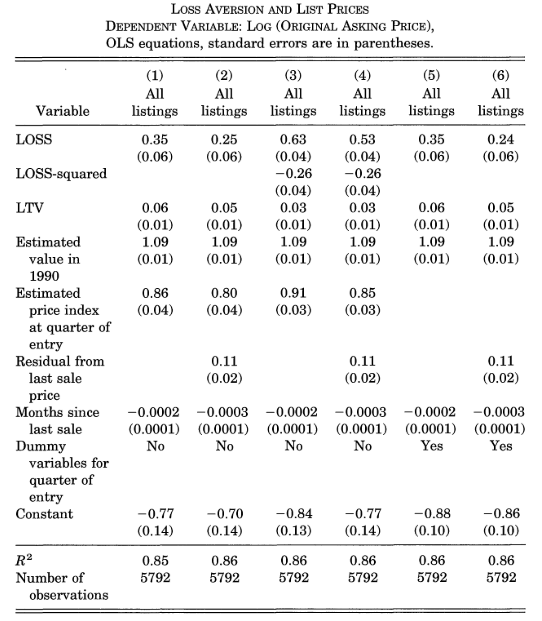
In Column (1) of the table, the statistically significant coefficient estimate for LOSS of 0.35 indicates that a 10% increase in a prospective loss leads a seller to set the asking price 3.5% higher, all else equal. The corresponding coefficient estimate for LOSS in Column (2) of 0.25 indicates that a 10% increase in a prospective loss leads a seller to set the asking price only 2.5% higher. Genesove and Mayer (2001) interpret the estimate from Column (1) as an upper-bound and that from Column (2) as a lower-bound on the true relationship between a prospective loss and the seller’s asking price. Similarly, the statistically significant coefficient estimate for LTV of 0.06 in Column (1) indicates that a 10% increase in the loan-to-value ratio for those sellers with ratios already above 0.8 leads these more highly indebted sellers to set an (upper-bound) asking price just over 6% higher, all else equal. Column (2) indicates that the lower-bound on the relationship between LTV and a seller’s asking price is 0.5%. Together, these results corresponding to LOSS and LTV indicate that sellers facing a loss on the sale of their apartment—both concerning their original purchase price and their loan-to-value ratio—exhibit a Disposition Effect by setting their asking prices above those set by sellers who do not face a loss.

So as not to shield buyers from their share of “Homo sapiensism” in the housing market—in particular Homo sapiens’ affinity for reference dependence—Simonsohn and Loewenstein (2006) investigated the US housing market between 1983 and 1993 to discern whether the average monthly rent or house price in the location where households moved from (i.e., their old locations) affected the monthly rent or house price they paid in the location they moved to (i.e., their new locations). In other words, do households that paid more for their housing in their old locations on average pay more for housing in their new locations. The authors find that the higher the rent or price paid in the old location, the higher the rent or price paid in the new location. Further, when households move for a second time within their new location, this positive relationship between prices paid in the old and new locations disappears. Simonsohn and Loewenstein conclude that households readjust their reference points after having lived in an area for some time. Therefore, the moral of Simonsohn and Loewenstein’s story is that even though Homo sapiens exhibit reference dependence in the housing market, at least their reference points are flexible.

Deal or No Deal?

When faced with an uncertain situation, do Homo sapiens set reference points based upon prior expectations, similar to how we set reference points in certain situations based upon prior experience? Post et al. (2008) set out to answer this question by assessing risky decisions made by 150 contestants from the Netherlands, Germany, and the US in the high-stakes game show Deal or No Deal.^[66] In the game, contestants choose among 26 briefcases, each containing some uncertain amount of money, ranging from €0.01 to €5 million (in the Dutch edition of the game). Each contestant selects one of the briefcases and thereafter owns its unknown contents. Next, he picks six of the remaining 25 briefcases to open. Each of the opened briefcases reveals a prize that is not in the contestant’s initially chosen briefcase. The contestant is then presented with a “bank offer” from the game’s host, which is the opportunity to walk away with a sure amount of money based loosely upon the average amount contained in the remaining unopened briefcases (Deal?), or to choose another five briefcases to open, followed by another bank offer (No Deal?). The game continues in this fashion until the contestant either accepts a bank offer or rejects them all and walks away with whatever amount of money is in the initially chosen briefcase.

Post et al. (2008) find that the typical contestant’s choices can be explained in large part by previous outcomes experienced during the game (e.g., the amounts of money in the opened briefcases and associated bank offers). Aversion to risk diminishes as prior expectations are either shattered by unfavorable outcomes (i.e., the opening of high-value briefcases) or surpassed by favorable outcomes (the opening of low-value briefcases)—known as Break-Even and House-Money Effects, respectively. This process of reference-point adjustment made by the contestant represents what the authors call path dependence, a form of dependence to which Homo economicus would never succumb.

Post et al.’s (2008) basic results for the Deal or No Deal contestants are presented in the table below. A contestant is labeled a Loser if his average remaining prize in the unopened briefcases (after having eliminated the lowest remaining prize) is among the worst one-third across all contestants in the same round of the game. A contestant is a Winner if his average remaining prize is among the highest one-third, and Neutral if neither a Loser nor a Winner. The column titled %BO lists the bank offer as a percentage of the money amounts in the remaining unopened briefcases per round, No. indicates the number of contestants who take the bank offer (i.e., take the deal) per round, and %D indicates the percentage of contestants who take the bank offer per round.

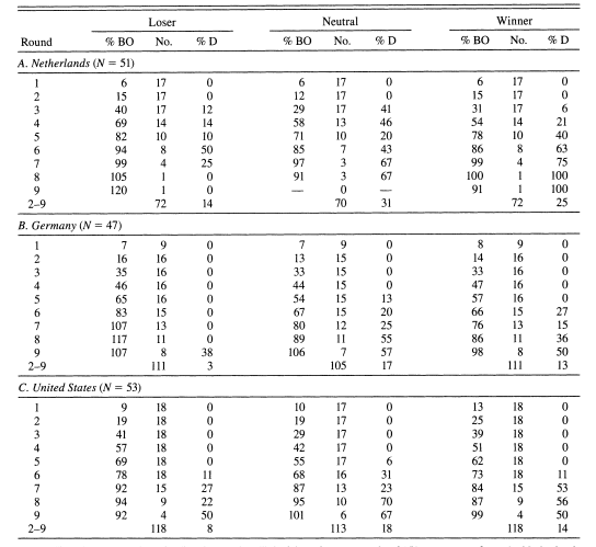
Focusing on the US sample of contestants (the results for the Netherlands and Germany samples are similar), we see that (1) %BO generally increases for each type of contestant (Loser, Winner, or Neutral) as the game progresses (i.e., the number of rounds increases), and (2) generally lower percentages of both Losers and Winners take the deal as compared to Neutrals as the game progresses. Overall, across rounds 2–9, 18% of all Deal or No Deal choices in the Neutral group are Deal, while only 8% and 14% of choices were Deal in the Loser and Winner groups, respectively. Post et al. (2008) interpret these results as evidence that risk aversion diminishes for both Losers and Winners, particularly for Losers, who have been unlucky in selecting which briefcases to open. Thus, prior outcomes are indeed an important reference points for risky choices.

Health Club Membership

What do we do when Homo sapiens are naive about their time-inconsistent preferences? Using attendance data for close to 8,000 health club members in New England from 1997–2000, DellaVigna and Malmendier (2006) were able to test whether members prone to making time-inconsistent choices choose a membership plan that helps them overcome this tendency most efficiently.^[67] In their sample, gym-goers have four different membership plans to choose from: (1) pay a $12 fee per visit, (2) pay $100 for a 10-visit pass, (3) sign an (automatically renewed, cancelable) monthly contract for unlimited visits at a standard fee of $85 per month, or (4) sign an annual contract (requiring in-person or in-writing renewal at the end of the contract) for unlimited visits at $850 per year. The authors find that, on average, members forego $600 in savings over the course of their memberships, indicating that they choose suboptimal membership plans given their attendance frequencies. DellaVigna and Malmendier attribute this suboptimality to optimistic overconfidence on the part of club members in terms of their future self-control or efficiency in attending the club. Sound familiar?

In particular, the authors find that members who choose a monthly membership pay on average 70% more than they would under the pay-as-you-go, fee-per-visit contract for the same number of visits. Eighty percent of these monthly members would have been better off had they paid per visit for the same number of visits. In addition, members who choose a monthly contract are 17% more likely to stay enrolled beyond one year than users committing upfront to an annual membership. Monthly members, therefore, end up paying higher fees for the option to cancel each month. Further, low-attendance members delay canceling their monthly contracts despite the small transaction costs of doing so.

Because of its automatic-renewal provision, the monthly contract’s default position is “opt-out,” meaning if a member decides to terminate the contract, she must opt out of it. By contrast, because of its non-automatic renewal provision, the annual contract’s default position is “opt-in,” whereby a member must opt into the contract on a yearly basis. In this way, the monthly contract is well suited for members who suffer from time inconsistency associated with procrastinating in joining the club, and then remembering to renew thereafter, while the annual membership better suits those members who have difficulty in motivating themselves to regularly attend the club for their workouts. For those members who end up attending less than they originally imagined they would, paying the per-visit fee is the best option. For those who follow through with attending often, the annual-fee membership seems to make the most sense. And for those who at the outset are unsure of how often they will attend, the monthly-fee membership seems best. DellaVigna and Malmendier (2006) investigate whether members choose the best membership plan for themselves at the outset and if not, then whether they learn and adjust to overcome their time-inconsistency problem.

The authors find that for monthly members there is not a month where their average price was beneath the standard $12 fee-per-visit or the $10 cost-per-visit associated with the 10-visit pass. On average, the price paid by the monthly members was above $17 per visit. Likewise, the average price paid by the annual members was above $15 per visit. Thus, on average, monthly and annual members are overconfident about their attendance at the club. They are not choosing their membership plans optimally.

Regarding the question of whether annual and monthly members learn and adjust to overcome their time-inconsistency problem, DellaVigna and Malmendier find that after the first year on an annual contract, the average annual member increases his monthly attendance to a point where the corresponding average price per visit falls from over $15 to approximately $11.30—lower than the $12 fee-per-visit, but still higher than the $10 cost-per-visit associated with the 10-visit pass. After the first six months on a monthly contract, the average monthly member decreases (yes, decreases) his monthly attendance to a point where the corresponding average price per visit rises to roughly $20 per visit. It appears that members with an annual membership adjust their attendance to an extent that mitigates the inefficiency of their choice but does not eliminate it. Members with monthly memberships, on the other hand, exacerbate the inefficiency of their choice. Alternatively stated, annual members learn to mitigate their time-inconsistency problem, while monthly members exacerbate theirs.^[68]

Lessons From an ‘All-You-Can-Eat’ Experiment

In Chapter 2, we were introduced to the notion of flat-rate pricing. Later, in Chapter 6, we encountered the Sunk Cost Fallacy. Conventional wisdom suggests that because All-You-Can-Eat (AYCE) restaurants charge a fixed price (i.e., flat rate) for a meal, the Sunk Cost Fallacy should be relatively easy to detect in Homo sapiens consumption behavior when they belly up to the buffet.

Because an AYCE customer faces zero marginal cost associated with additional amounts of food consumed, the rational model of Homo economicus suggests that he should continue to eat until the marginal utility of consumption reaches zero. This is because the per-unit cost of consumption continually decreases with the amount consumed. Once the AYCE customer has paid the fixed price for the meal, his budget constraint on added consumption is effectively obviated. The only thing stopping him now is his epidemiological and neurological impulses. As Just and Wansink (2011) point out, in an AYCE setting price can influence whether one chooses to eat at the restaurant, but it should not affect the amount of food one consumes once he has chosen to eat there.

As we know, some Homo sapiens are driven to “get their money’s worth” in various situations (recall the experiments in Chapter 6 involving the choice of whether to drive through snowstorms and rainstorms to get to a sporting event). In other words, Homo sapiens are susceptible to the Sunk Cost Fallacy. To the extent that the flat-rate pricing of AYCE restaurants triggers the Sunk Cost Fallacy in their customers, increasing the price of an AYCE buffet should increase the amount of food a customer ultimately eats. Just and Wansink test this hypothesis by designing an innovative field experiment that assigned customers to one of two prices at an AYCE pizza buffet restaurant.^[69] The authors find that those assigned to the higher-price treatment consumed just under 40% more pizza than those assigned to the lower-price treatment. In other words, a higher flat rate did indeed increase the amount of food consumed. But is it a Sunk Cost Fallacy that drove these results, or perhaps an alternative effect?

Permission to conduct the experiment was granted by the Pizza Garden, an AYCE restaurant located one mile south of Champaign, Illinois. The experiment was conducted during the restaurant’s exclusive lunch buffet hours on a Tuesday, Wednesday, and Thursday in early April 2005. Members of the experiment’s control group paid for the pizza buffet at the regular price of $5.98, while members of the treatment group were given coupons for 50% off this regular price. A total of 66 subjects participated in the experiment.

As Just and Wansink point out, customers choosing to eat at this restaurant would have already decided to eat the buffet at the regular price. In fact, no individuals included in either the treatment or control group failed to purchase the pizza buffet. While in the restaurant, pizza consumption was measured by three assistants who served as hostesses. The assistants were blind to the purpose of the study and had no knowledge of which patrons had been randomly assigned to the control or treatment groups. The assistants noted how many pieces of pizza each customer brought back from the buffet table, and how much was left uneaten after each customer completed their meal. Because the assistants were also responsible for busing tables, collecting the uneaten food was possible to do without raising suspicion. Uneaten pizza was weighed in a back room to more accurately assess what percentage of the pizza taken from the buffet table was actually eaten. After paying for their meals, the experiment’s participants completed a short questionnaire concerning their demographics, how much they believed they ate, and their quality assessments of the pizza. The size of the group each participant was a part of while eating their meal was also noted, as group size can be a determinant of how much an individual eats at a restaurant.

The authors find that, on average, participants paying the full price ate roughly one slice more than participants paying half price, which nevertheless resulted in the full-price participants paying roughly $0.58 more per slice than the half-price participants. Full-price participants also left more uneaten pizza on their plates as food waste. Therefore, Just and Wansink find evidence that higher prices do indeed lead to greater pizza consumption. The Sunk Cost Fallacy seems to be in play at AYCE restaurants.

The Persistence of Political Misperceptions

Political misperceptions have probably existed for as long as Homo sapiens have practiced politics. Although their frequency, intensity, and the extent to which they are disseminated among the general public via social media outlets are worthy of concern, misinformation campaigns (and the unsubstantiated conspiracy theories they spawn) have a long history in worldwide politics.

In a series of field experiments with self-identified ideological subgroups of adults, Nyhan and Reifler (2010) investigated the extent to which corrective information embedded in realistic news reports can succeed in reducing prominent misperceptions about contemporary political issues (according to the authors, misperceptions occur when people’s beliefs about factual matters are not supported by clear evidence and expert opinion—a definition that includes beliefs about the world that are both false and unsubstantiated). In each of the experiments, the subgroups failed to update their beliefs when presented with factually corrective information that runs counter to their ideological predispositions. In several instances, the authors find that the corrections actually strengthen (yes, strengthen) rather than weaken misperceptions among those most strongly tied to their predispositions.

Nyhan and Reifler premise their experiments on previous research showing that many citizens base their policy preferences on false, misleading, or unsubstantiated information related to their political ideologies and what they believe to be true. For instance, after the US invasion of Iraq in 2003, the belief that Iraq had stockpiled weapons of mass destruction prior to the invasion was closely aligned with one’s level of support for President Bush. As the authors point out, people are typically exposed to corrective information within objective news reporting, pitting two sides of an argument against each other. Nevertheless, we Homo sapiens are likely to resist or reject arguments and evidence contradicting our opinions.

Specifically, Nyhan and Reifler test three hypotheses about the extent to which corrective information overrides, or at least tempers, the effect of a subject’s political ideology:

• Hypothesis 1. The effect of corrective information on misperceptions will be moderated by political ideologies.
• Hypothesis 2. Corrective information will fail to reduce misperceptions among the ideological subgroup that is likely to hold the misperception.
• Hypothesis 3. In some cases, the interaction between corrective information and political ideology will be so strong that misperceptions will actually increase for the ideological subgroup in question. Ouch. This is known as a Backfire Effect.

In the experiments, subjects read mock newspaper articles containing a statement from a political figure who reinforced a widespread misperception concerning the war in Iraq, tax cuts, or stem cell research (three popular issues at the time in American politics). Subjects were randomly assigned to read articles that either included or did not include corrective information immediately after a false or misleading statement.

The first experiment tested the effectiveness of corrective information embedded in a news report on beliefs that Iraq had stockpiled weapons of mass destruction (WMD) immediately before the US invasion. As Nyhan and Reifler point out, one possible explanation for why this misperception persisted was that journalists had failed to adequately fact-check Bush administration assertions that the US had found WMDs in Iraq. Another was people’s fear of death in the wake of the September 11, 2001, terrorist attacks, known as “salience of mortality.”

Subjects were instructed to read a mock news article attributed to the Associated Press that reported on a Bush campaign speech in Pennsylvania in October 2004. As Nyhan and Reifler describe it, the article describes Bush’s remarks as a rousing, no-retreat defense of the Iraq War. The article included a quote from Bush: “There was a risk, a real risk, that Saddam Hussein would pass weapons or materials or information to terrorist networks after September 11th, that was a risk we could not afford to take (page 312).” A control group received only this information, while one treatment group also received corrective information based upon the Duelfer Report, which documented the lack of both Iraqi stockpiles of WMDs and an active production program immediately prior to the US invasion. Another treatment group received a mortality-salience question: “Please briefly describe the emotions that the thought of your own death arouses in you. Jot down, as specifically as you can, what you think will happen to you as you physically die and once you are physically dead.”

All subjects were then asked to state whether they agreed with the summary statement: “Immediately before the US invasion, Iraq had an active weapons of mass destruction program, the ability to produce these weapons, and large stockpiles of these weapons, but Saddam Hussein was able to hide or destroy these weapons right before US forces arrived.” Responses were measured on a five-point Likert scale ranging from 1 = “strongly disagree” to 5 = “strongly agree.” To gauge a subject’s ideological disposition, subjects self-identified according to a centered seven-point Likert scale, ranging from -3 = “strongly liberal” to 3 = “strongly conservative.” An additive five-question scale measuring political knowledge used conventional factual questions.

As the results in the table below demonstrate, Nyhan and Reifler find that, as expected, more knowledgeable subjects were less likely to agree with the summary statement (the coefficient estimates for Political Knowledge of -1.133 and -1.081 are statistically significant), conservatives were more likely to agree with the statement (the coefficient estimates for Ideology of 0.347 and 0.199 are also statistically significant), but neither the corrective information (Correction) nor mortality salience question (Mortality Salience) had statistically significant effects on subjects’ responses.^[70]

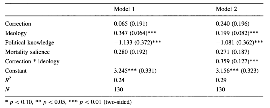
In Model 2, the introduction of the interaction term Correction*ideology tests whether the effect of the corrective information is moderated by subjects’ political ideologies (Hypothesis 1), in particular whether the corrective information will be increasingly ineffective as subjects’ political ideologies increase their susceptibility to misperception—in the case of justifying the Iraq War among politically more conservative subjects (Hypothesis 2)—or whether the corrective statement will backfire and that misperceptions will actually increase among politically conservative subjects (Hypothesis 3). Because the coefficient estimate on this interaction term is positive and statistically significant, it supports each of the three hypotheses. Looking more closely at their data, the authors find that the corrective information worked as expected. When exposed to the corrective information, very liberal subjects became more likely to disagree with the summary statement. No statistical effect was found for subjects describing themselves as liberal, somewhat left of center, or centrist. And conservatives became more likely to agree with the summary statement…kaboom, corrective information backfired!

The authors go on to test whether the Backfire Effect occurred because conservative participants distrusted the news source, Associated Press. They find that news source (New York Times vs. Fox News) has no impact on the result. Interestingly, when the context of the mock news article is changed from the 2004 Bush campaign speech to a 2005 Bush statement about Iraq, the Backfire Effect not only disappears in general, but transforms into a Forward-Fire Effect—conservatives receiving the corrective statement are less likely to agree with the summary statement. This is evidence of a framing effect. Nevertheless, among those subjects who rated Iraq as the nation’s “most important problem,” the Backfire Effect persisted with the 2005 Bush statement about Iraq.

Nyhan and Reifler put forth two possible justifications for the Forward-Fire Effect. They point out that conservatives may have shifted their rationale for supporting the war in tandem with the Bush administration, which over time sought to distance itself from the WMD rationale for the war. By early 2006, national polls suggested a decline in Republican beliefs that Iraq had stockpiled WMDs before the US invasion. Another possible explanation is that conservatives generally placed less importance on the war by early 2006, and thus were less likely to counterargue the corrective information.

Lastly, the authors found a similar Backfire Effect when the issue at hand was misperceptions about the Bush tax cuts of 2001 and 2003. Regarding the issue of misperceptions regarding stem cell research in the early 2000s—a misperception held among liberals—Nyhan and Reifler find that corrective information worked (i.e., had a statistically significant negative effect on misperceptions) among subjects self-identifying as centrists and right-of-center, but failed to affect subjects identifying as liberal (i.e., left-of-center and beyond). Thus, in this experiment evidence is found in favor of Hypotheses 1 and 2, but not Hypothesis 3 concerning stem cell research. Thankfully, stem cell research is not an issue inspiring a Backfire Effect among liberals.

Temptation and Self-Control – The Case of Potato Chips

As Wertenbroch (1998) observes, we Homo sapiens often cave in to temptation (e.g., about the consumption of “vice goods” such as cigarettes, as opposed to “virtue goods” such as reduced-fat yogurt) against our own better judgment and self-interest. In dealing with temptation, realizing immediate utility from consumption conflicts with the longer-term utility associated with self-control. Self-rationing is a form of self-control that limits a consumer’s stock of vice goods and thus the possibility of consuming them. Self-rationing imposes transactions costs on additional consumption and is perhaps an expression of attendant feelings of guilt. One way to test the extent of a consumer’s self-control is to answer the question, Are consumers less likely to purchase larger quantities of a vice good than a virtue good in response to equal unit-price reductions? If the answer to this question is “yes,” then consumers exhibit self-control in the face of temptation.

Using an experimental market approach, Wertenbroch tests whether vice consumers are less price sensitive than virtue consumers by examining consumers’ demands for potato chips at two different quantity-discount price depths offered for a large-purchase quantity. The potato chips are framed as either 25% fat (relative vice good) or 75% fat-free (relative virtue good). Approximately 300 MBA students at Yale University participated in the experiment. The subjects were first shown a 6-oz. bag of an existing brand of potato chips as a reference package size. A questionnaire then offered them the opportunity to buy zero, one, or three 6-oz. bags of a new brand of potato chips at different prices per bag—$1 for a single bag and $2.80 for three bags (if the subject had been randomly assigned to the “shallow discount” treatment group), or $1.80 for three bags (if randomly assigned to the “deep discount” treatment group). A single bag represents the small size and three bags represent the large size. The new brand was described as having an innovative mix of ingredients and as currently being test marketed.

Subjects were informed that approximately one in 10 of those who completed their questionnaires would be randomly selected in a lottery to receive $10 in compensation for agreeing to participate in the experiment. To ensure that subjects would accurately reveal their demand for the chips, they were informed that the lottery winners would have to purchase (out of their $10 compensation payment) the respective amounts of potato chips they had chosen in the questionnaire at the given prices.

Wertenbroch finds that subjects who bought potato chips were more likely to prefer the large size when the chips were framed as 25% fat (again, the vice good) than as 75% fat-free (the virtue good). However, the probability of buying the large size under the virtue frame increased from 20% under the shallow discount to 65% under the deep discount (i.e., an increase of 225%). Under the vice frame, the corresponding increase was from 41% to 53%, an increase of merely 29%. Therefore, as the author points out, increasing the depth of the quantity discount was less effective in enticing vice consumers to increase their purchase quantities, suggesting that they self-imposed a rationing constraint as external price constraints were relaxed.^[71]

Dishonesty’s Temptation

According to the National Retail Federation (NRF), customer and employee theft, fraud, and losses from other “retail shrink” in the US totaled just under $62 billion (or approximately 1.6% of total sales) in 2019, representing a 22% increase over the previous year (NRF, 2020). You read that correctly, $62 billion, with a “b.” Interpreting retail shrink as the aggregation of consumers being dishonest with the businesses that supply our retail goods and employees being dishonest with the businesses that employ them, this $62 billion can be thought of as representing the monetary cost of dishonesty in the retail sector of the economy.^[72]

Let’s face it. Dishonesty is an inexorable part of the human experience, so inexorable that even Homo economicus can be expected to be dishonest in any given situation when the coldly calculated expected benefit of dishonesty outweighs its expected cost. To demonstrate dishonesty’s pervasiveness among Homo sapiens (or, as Mazar et al. (2008) describe it, to measure the extent to which a little bit of dishonesty yields profit without spoiling one’s positive self-view) Mazar et al. conducted a series of experiments enabling a comparison between the performance of participants in control conditions (in which the participants had no opportunity to be dishonest) with “cheating conditions” (in which participants had the latitude to cheat).

In the first experiment, the authors tested whether reminding participants of their standards for honesty would induce greater levels of honesty among them than among participants who were not preempted with such reminders. Over two hundred MIT and Yale students participated in the experiment, which consisted of multiple paper-and-pencil tasks appearing together in a booklet. To begin, participants were asked to either write down the names of 10 books they had read in high school (no moral reminder) or the Ten Commandments (moral reminder) within a two-minute time limit.^[73] Next, the participants were provided with a test sheet and an answer sheet. The test sheet consisted of 20 matrices, each based upon a set of 12 three-digit numbers. Participants had four minutes in which to find two numbers per matrix that added up to 10. An example matrix is depicted below.

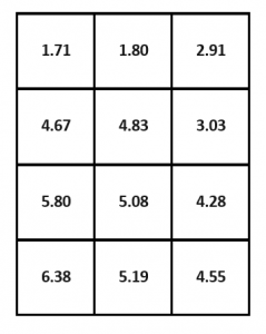
The answer sheet was used by a participant to report her total number of correctly solved matrices. At the end of the session, two randomly selected participants earned $10 for each correctly solved matrix.

At the end of the four-minute matrix task, the experimenter verified each participant’s answers. Participants in the experiment’s two treatment (or recycle) groups indicated the total number of correctly solved matrices on their answer sheets, and then tore out the original test sheets from the booklet and placed them in their belongings (to recycle on their own later), thus providing these groups of participants with an opportunity to cheat.

The results from this experiment were as anticipated. The type of reminder (10-books vs. Ten Commandments) did not affect the average participant’s performance in the two control conditions—each group averaged just over three correctly solved matrices—suggesting that type of reminder influenced neither ability nor motivation. However, in the two treatment conditions, reminder type mattered. Following the 10-book recall task, participants self-reported an average of slightly more than four correctly solved matrices (which was significantly higher statistically than the control groups’ three-matrix average), thus pointing to the likely presence of cheating among this group of participants. To the contrary, participants in the Ten Commandment recall task self-reported an average of slightly less than three correctly solved matrices (which was not significantly different statistically than the control groups’ averages). Mazar et al. conclude that reminding participants of standards for morality eliminates cheating.

In the second experiment conducted with over 200 MIT and Yale students, the Ten Commandments recall task was replaced with an Honor Code treatment, the 10-book recall task was eliminated, and payments for correctly solved matrices (for randomly chosen participants) were either 50 cents or $2 per matrix (to test for possible payment-level effects). In the two control groups, participants again handed both the test and answer sheets to the experimenter at the end of the matrix-solution task. The experimenter verified their answers and wrote down the number of correctly solved matrices on the answer sheet. In the two recycle treatments (one without any recall task, henceforth, “recycle” treatment, the other with the Honor Code recall task, henceforth, “recycle+HC”) participants indicated the total number of correctly solved matrices on the answer sheet, folded the original test sheet, and then placed it in their belongings, similar to the first experiment. In the recycle+HC treatment, there was a statement located at the top of the matrices test sheet that read: “I understand that this short survey falls under MIT’s [Yale’s] honor system (page 637).” Participants printed and signed their names below the statement.

Results from this experiment are depicted in the figure below. Similar to the results for the first experiment, we see that while the recycle treatment resulted in a statistically significant increase in self-reported correctly solved matrices relative to the control groups and recycle+HC treatments (the whiskers do not overlap), the control groups and recycle+HC treatments did not result in statistically different scores. Interestingly, the different payment amounts (50 cents and $2) did not result in different scores within each respective group type—control, recycle, or recycle+HC.

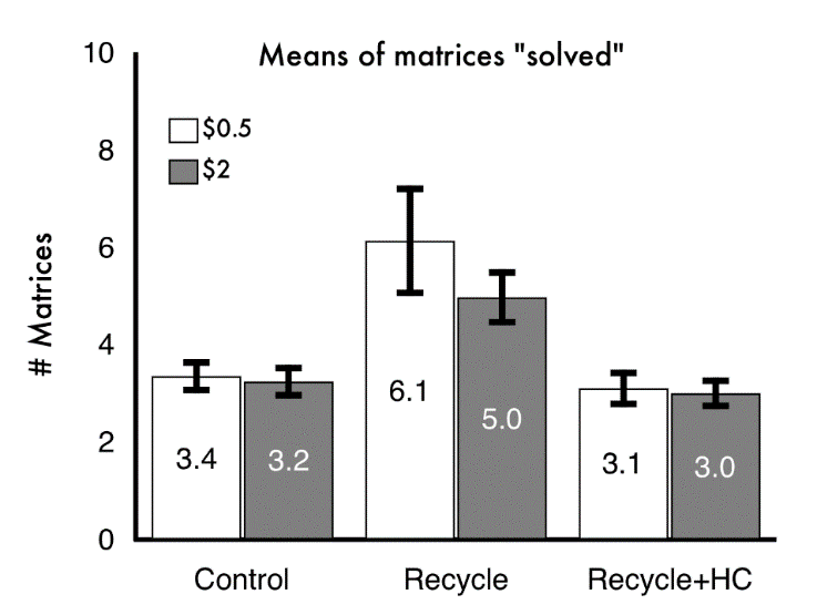
Lastly, in a third experiment, Mazar et al. tested whether the opportunity for dishonest behavior occurred in terms of money or in terms of an intermediary medium (tokens). The authors posited that introducing tokens would offer participants more latitude in interpreting their actions, hence making it easier for participants to justify cheating. Participants (450 MIT and Yale students) had five minutes each to complete the matrix task and were promised 50 cents for each correctly solved matrix. The same control and recycle treatment as in the second experiment were used, along with a “recycle+token” treatment where participants knew that each (self-reported) correctly solved matrix earned one token, which could be exchanged for 50 cents a few seconds later.

Similar to their previous findings, Mazar et al. found that the average participant in the recycle treatment reported having solved significantly more matrices than the average participant in the control group, suggesting the presence of dishonesty among the former group. Interestingly, introducing tokens as the medium of immediate exchange further increased the magnitude of dishonesty in the recycle+token treatment, such that it was significantly larger than that exhibited in the recycle treatment. This leads the authors to conclude that a medium, such as tokens, facilitates dishonesty, which helps explain the high levels of employee theft and fraud (e.g., stealing office supplies and merchandise, and putting inappropriate expenses on expense accounts) found in the US retail industry. As Ariely (2008) puts it, “what a difference there is in cheating for money versus cheating for something that is a step away from cash!” (page 299)^[74]

Bigger Universities, Smaller Silos

In Chapter 1, the concept of homophily and the Silo Effect were briefly explored. Left unanswered was the question of how the size and diversity of social choices (i.e., social ecology) affect the similarities between relationship partners (i.e., the extent of homophily existing between the two). As Bahns et al. (2010) point out, the initiation of an interpersonal or inter-organizational relationship is not only a dyadic process. The process is also influenced by the broader group of social contacts present in the local environment. It is the social ecology that shapes the kinds of communication and interactions that occur between the two partners, potentially hardening or softening the pretext for a silo effect.

Bahns et al. aver that, in general, when Homo sapiens have a choice, they tend to initiate and build relationships with partners who are similar to them. In their study, they compare the degree of similarity within dyads in a particular social ecology—a college campus—that varies in the size of the available pool of relationship choices. The authors compare dyads formed among students in public settings at a large state university to dyads formed in the same way in smaller colleges in the same state. Because students located at the larger universities can choose among a greater variety of fellow students, Bahns et al. hypothesize that these students will also be able to match their interests and activities more closely with partners than students located at smaller universities, which leads to a straightforward, albeit ironic, hypothesis. Greater human diversity within an environment leads to less personal diversity within dyads.

To test this hypothesis 110 students (55 dyads) were recruited from a large campus (the University of Kansas) and 158 students (79 dyads) from four small universities located in small eastern and central Kansas towns. To collect their data, experimenters visited each campus on a midweek day and located a public space where students were interacting with each other (e.g., the student union and a cafeteria). Naturally occurring dyads, which were randomly identified, were defined as any group of exactly two people who appear to be interacting in some way. The experimenter then administered a five-section questionnaire.

The first section gathered information about the students’ socio-demographics and the nature of their relationship (e.g., how long they had known their dyad partner, how close they were, and how many hours per week they spent with the partner). The second section of the questionnaire asked about different social attitudes concerning abortion, religious observance, birth control, the importance of maintaining traditional husband-wife roles in a marriage, and capital punishment. The third section measured what the authors call “feeling thermometers” of attitudes toward/prejudices against five different social groups—Arabs, Black Americans, overweight people, gay men, and Jews. The fourth section measured health-related behaviors (e.g., tobacco use, alcohol use, and exercise). The fifth section measured the extent of agreement with what the authors call relational mobility statements, i.e., (1) “At this school, it is easy to meet new people,” (2) “People at this school have few chances to get to know new people,” (3) “It is common for me to see people on campus who are unfamiliar” (page 123), and psychological independence statements, i.e., (1) “If a person hurts someone close to me, I feel personally hurt as well,” (2) “My close relationships are unimportant to my sense of what kind of person I am,” and (3) “Even when I strongly disagree with group members, I avoid an argument” (page 124).

Bahns et al. find that dyads on the smaller campuses reported less relational mobility, implying greater perceived relationship opportunities on the large campus. However, no evidence is found that distinguishes the degree of psychological independence across the large and small universities. Similarly, there was no statistically significant difference across universities regarding length of relationships and amount of time spent together. However, dyads from the smaller universities rated their relationships as being closer than those from the large university.

Participants from small universities reported somewhat more conservative political beliefs, more prejudice toward Black people, more negative attitudes toward abortion, and more positive attitudes toward religion compared to participants from the large university. Participants from the large university exercised less, drank more alcohol, and smoked more tobacco than participants from the small universities.

The authors conclude that attitudes and behaviors are meaningful and important dimensions of social relationships in both social ecologies—students sort into dyads along these lines. Most importantly for this study, Bahns et al. find significantly greater degrees of similarity within dyads formed at the large university than at the small universities in terms of socio-demographics and social attitudes. In other words, greater diversity within the university environment leads to less personal diversity within dyads. As the authors state,

“It cannot be surprising that size of opportunity leads to the ability to fine-tune the outcome. When opportunity abounds, people are free to pursue more narrow selection criteria, but when fewer choices are available, they must find satisfaction using broader criteria” (p. 127).

Tipping Points

To the extent that a given population of Homo economicus is comprised of risk-averse vs. risk-neutral vs. risk-loving individuals (and those whose (time-consistent) discount rates are relatively small vs. relatively large), tipping points like those explored in Gladwell (2002) are possible in a variety of social settings, such as the spread of disease (e.g., HIV/AIDs and syphilis), crime (e.g., use of crack cocaine and Methamphetamines), fashion trends (e.g., wearing of Hush Puppy and Airwalk shoes), popular children’s shows (e,g., Sesame Street and Blues Clues), and new technologies (e.g., fax machines and cellular phones) in epidemic (or geometric) proportions. Throw in Homo sapiens’ predispositions for reference dependence, loss aversion, and the many effects and biases encountered in Chapters 1 and 2, and the proverbial stage is set for tripping over the myriad of tipping points lurking out there in the real world.

As Gladwell points out, three interconnected characteristics underpin the spread of epidemics: (1) contagiousness of the micro-organism, fad, idea, or behavior in question, (2) the dependence of big effects on relatively small causes, and (3) the suddenness of change (i.e., the presence of tipping points). Particularly when it comes to epidemics depending upon word-of-mouth, these characteristics can also be thought of, roughly and respectively, as (1) the “stickiness factor” of an initiating message, (2) the “law of the few” individuals with rare social gifts, and (3) the “power of context” (i.e., the recognition that Homo sapiens are quite sensitive to their environments).

Gladwell specifies the Law of the Few as consisting of a confluence of three types of individuals: connectors (gregarious and intensely social individuals who know lots of other people from different walks of life, more as acquaintances than friends); mavens (information specialists who not only gather information but also revel in the opportunity to spread the information to others); and salesmen (those with the ability to persuade others who are unconvinced about what they are hearing from mavens and connectors).

According to Gladwell, the power of context relates to the subtle, hidden, and often unspoken messages or cues that are transmitted in the run-up to a tipping point. This implies that an individual’s behavior is, to varying degrees, a function of social context. In the case of crime, for example, subtle messages sent by broken windows in a community or graffiti and broken turnstiles in a subway station help create a social context suggesting that it is ok to commit crime here.

Messages, both spoken and unspoken, are sticky when they are memorable and ultimately compel the recipient of the message to take a targeted action. Stickiness in this sense relates to a message’s effectiveness, similar to the previously encountered messages designed to reduce littering, environmental theft, drunk driving, and to promote energy conservation and better health care.

Gladwell provides several examples of epidemics that have adhered to the patterns identified above (e.g., contagiousness, dependence of big effects on relatively small causes, and the presence of tipping points). These examples include the massive and rapid-fire success of the late 1960s children’s educational TV show Sesame Street (and the show it later spawned in the mid-1990s, Blue’s Clues), the direct-marketing campaign of the Columbia Record Club in the 1970s, the surge of crime and its subsequent reversal on the NY City subway system in the mid-1980s, adoption by US farmers of new hybrid seeds in the late 1930s, teenage suicide in Micronesia in the mid-1960s through the 1980s, and even Paul Revere’s midnight ride at the outset of the American Revolutionary War in the late 1700s.

Consider the epidemic of teenage smoking in the US. Gladwell ascribes primary billing in this epidemic’s cause to salespeople (recall the law of the few), in particular extroverts, individuals who tend to be more rebellious and defiant and who make snap judgments and take more risks. These are people who are not perceived as being cool because they smoke, rather they smoke because they are cool. In effect, this epidemic’s salespeople are also its tipping points, or “tipping people.” Adolescents are naturally drawn to them.

According to Gladwell, the epidemic’s stickiness factor occurs naturally. Because the smoking experience is so memorable and powerful for certain people, they cannot stop smoking—the habit sticks. Whether a teenager picks up the habit depends upon whether he comes in contact with a salesperson who effectively gives the teenager permission to engage in deviant acts. Of course, whether a teenager likes smoking cigarettes enough to keep using them depends upon a very different set of criteria. As Gladwell points out, nicotine is highly addictive but only in some people some of the time. Millions of Americans manage to smoke regularly and not get hooked. For these individuals, smoking is contagious but not sticky.

What to do? Gladwell suggests we might attack the epidemic from different, albeit self-enforcing, angles. One angle would be to prevent the salespeople from smoking in the first place. Another would be to convince all those who look to salespeople for permission to smoke that they should look elsewhere, to get their social cues from non-smoking adults. Further, as with other neurologically triggered addictions, zeroing in on combatting depression among teenagers would enable the exploitation of a critical vulnerability in the addiction process.

Regardless of which angle is emphasized in the effort to countervail the profuse tipping points in teenage smoking, it is never too late to consider new approaches in the campaign to control the epidemic. According to the American Lung Association (2020), every day, almost 2,500 children under 18 years of age try their first cigarette, and more than 400 of them will become new, regular, daily smokers. Of adolescents who have smoked at least 100 cigarettes in their lifetime, most of them report that they would like to quit but are unable to do so. If current tobacco use patterns persist, an estimated 5.6 million of today’s youth under 18 will die prematurely from a smoking-related disease.

Magical Thinking

It is (hopefully) safe to say that the majority of Homo sapiens distinguish both themselves and Homo economicus from superheroes (Homo vir fortis)—those with magical powers. However, the extent to which we Homo sapiens engage in magical thinking from time-to-time is perhaps less distinguishable. As Pronin et al. (2006) puts it,

“Every so often, we may learn that someone we have wished ill actually has become ill, or that the sports team for which we are cheering has in fact gone and won the game. When such things happen, although we are far from causal, we may nonetheless experience a sense of authorship—a feeling that we caused the events we had imagined” (p. 218).

To investigate the prevalence of this type of magical thinking, the authors designed experiments to examine whether and when such experiences of everyday magic might arise.^[75] They propose the formal hypothesis that belief in one’s own magical powers can arise when we infer that we have personally caused events based upon perceiving a relation between our thoughts and subsequent events. One experiment tests whether college students might come to believe that they have caused another person pain through a voodoo curse when they have thoughts about the person consistent with such harm.

In this experiment, participants assumed the role of “witch doctor” in an ostensible voodoo enactment involving a confederate (a role-playing experimenter) as their “victim.” The authors arranged for participants to encounter either a victim who was offensive (henceforth evil) or one who was neutral. Following this encounter, participants were instructed to stick pins in a voodoo doll representing the victim, in the victim’s presence. The victim subsequently responded by reporting a slight headache, and participants were queried about their reactions to this reported symptom. The experiment made possible the investigation of whether participants who harbor evil thoughts toward a victim are more likely than neutral-thinking participants to perceive that they caused the victim harm.

Slightly fewer than 40 residents of Cambridge, MA were randomly assigned to either a neutral-thoughts condition or an evil-thoughts condition. Each participant and confederate (a 22-year-old man) was greeted in a waiting area by the experimenter and escorted to the laboratory. The participant and confederate were seated at a table with a handmade twig-and-cloth voodoo doll lying on it. The experimenter explained that the experiment was designed to assess psychosomatic symptoms and physical health symptoms resulting from psychological factors, and that the study was investigating this question in the context of Haitian Voodoo. For background, the experimenter furnished both individuals with an abridged version of Cannon’s (1942) Voodoo Death. This scientific account of how voodoo curses might impact physical health was included to bolster the plausibility of curse effects.

In the condition designed to induce evil thoughts, the confederate arrived at the experiment 10 minutes late, thus keeping the participant and experimenter waiting. When the experimenter politely commented that she was really glad he made it, he muttered with condescension: What’s the big deal? He wore a T-shirt emblazoned with the phrase Stupid People Shouldn’t Breed, and he chewed gum with his mouth open. When the experimenter informed the participant and confederate that they had been given an extra copy of their consent form to keep, the confederate crumpled up his copy and tossed it toward the garbage can. He missed, shrugged, and left it on the floor. Finally, while he and the participant read the Voodoo Death article, he slowly rotated his pen on the tabletop, making a noise just noticeable enough to be grating. Post-experiment interviews indicated that participants in the evil-thoughts condition were cognizant of many of these annoyances and found themselves disliking the confederate. Although the confederate was, by design, aware of these adjustments in his behavior, he was otherwise uninformed about the study’s hypotheses.

After reading Voodoo Death, the participant and confederate were each asked to pick slips from a hat to determine who would be the witch doctor and who would be the victim. Both slips were labeled witch doctor, but the confederate pretended that his said victim. The confederate victim was then asked to write his name on a slip of paper to be affixed to the doll. Both victim and witch doctor then completed a page entitled Baseline Symptom Questionnaire that asked them to indicate whether they currently had any of 26 physical symptoms (e.g., runny nose, sore muscles, and/or headache). The confederate circled “No” for each symptom. To ensure that the participant knew the victim’s purported health status, the experimenter verbally confirmed that the victim currently had no symptoms.

The experimenter then informed both individuals that reported cases of voodoo suggest that the witch doctor should have some time alone to direct attention toward the victim, and away from external distractions (before invoking the curse by pricking the voodoo doll), and she escorted the victim from the room. The participant was then asked to generate vivid and concrete thoughts about the victim but not to say them aloud. Afterward, the experimenter returned with the victim, who was again seated across from the participant. The participant was instructed to stick the five available pins into the doll in the locations of the five major weaknesses of the body: the head, heart, stomach, left side, and right side. Once the participant completed this task of piercing the doll, the victim was asked to complete a second symptom questionnaire (identical to the first). However, this time the victim invariably circled one symptom: a headache. He elaborated at the bottom of the page: I have a bit of a headache now. When asked to confirm this symptom, he averred with a slightly uncomfortable facial expression and the response “Yeah.” The experimenter then stated that she would like to take some time with the victim to question him in detail about his symptoms but that she would first quickly ask the witch doctor some questions about his or her experiences in the experiment.

With the victim escorted from the room, the witch doctor was asked the following six questions:

1. “Did you feel like you caused the symptoms that the ‘victim’ reported, either directly or indirectly?”
2. “Do you feel that your practice of voodoo affected the victim’s symptoms?”
3. “How much do you feel like you tried to harm the victim?”
4. “Do you feel that sticking the pins in the doll was a bad thing to do?”
5. “Did any negative thoughts about the victim pop into your head during the minute you had to yourself before the voodoo exercise?”
6. “Did you have any negative thoughts toward the victim before (or while) you did the pin pricks?” (p. 221)

Pronin et al.’s results were as expected. Witch doctors in the evil-thoughts condition were successfully induced to think ill of their victim; they reported significantly more negative thoughts about the victim than those in the neutral-thoughts condition. Most importantly, witch doctors in the evil-thoughts condition were more likely than those in the neutral-thinking condition to believe that they had caused the victim’s headache. Witch doctors prompted to think evil thoughts reported feeling no more guilt than those prompted to think more neutrally about their victim. The authors conjecture that witch doctors saw the victim’s headache as a just reward for his unpleasant behavior, and so they were not upset at having caused him pain. Ouch!

Concluding Remarks

As mentioned in this section’s Introduction, the empirical studies and field experiments discussed here exemplify how behavioral economists have tested for the existence of the biases, effects, and fallacies underpinning Homo sapiens’ choice behaviors, as well as the extent to which different implications of Prospect Theory (e.g., loss aversion, reference dependence, and the endowment effect), hyperbolic discounting, and mental discounting help explain these behaviors. Several of the case studies examined in this section also broach a host of contexts in which Homo sapiens exhibit socially degenerative behaviors (such as racial discrimination, criminal behavior, time-inconsistency, deadweight gift-giving, and procrastination), and empirically measure the extent of these behaviors in real-world situations.

Thankfully, the proverbial story does not stop there. Several of this section’s case studies examine what Thaler and Sunstein (2009) call “nudges” to correct degenerative behaviors. For example, we explored ways in which the design of default options can be used to save lives, the extent to which basic-income and microfinance programs can help alleviate poverty, the extent to which simply raising awareness can help reduce racial discrimination, and how monetary reward/punishment schemes and information campaigns can (at least to some extent) mitigate social ills such as homelessness, food waste, and drunk driving, and promote improvements in such areas as energy conservation, public health, income tax compliance, and voter turnout. These types of nudges are the bridges between what behavioral economics teaches about Homo sapiens’ quirks and consequent choice behaviors, on the one hand, and public policies that, with varying degrees of success, reorient these choice behaviors for the social good.

The number of organizations that have formed during the past decade to promote public policies incorporating insights from behavioral economics (i.e., to nudge) is impressive. For example, The Behavioral Insights (BI) Team began as a small agency of the United Kingdom’s (UK’s) government whose mission was to design innovative nudges to improve the workings of British society. Today the BI team is a global social purpose company whose projects span over 30 different countries. The BI Team’s policy areas include finance, crime and justice, education, energy, the environment and sustainability, health and well-being, international development, taxation, and work and the economy.

GreeNudge is a Norwegian non-profit organization focusing on Norway’s health-care system, specifically how to nudge consumers to choose healthier and more environmentally friendly foods in grocery stores, and, through an effort called Behaviourlab, apply behavioral science toward the realization of the United Nation’s 17 Development Goals. In Peru, the nation’s Ministry of Education has established MineduLAB, a laboratory designed to leverage lessons from behavioral economics to improve the country’s educational policies. And the World Bank’s Mind, Behavior, and Development Unit (eMBeD) is the spearhead of a worldwide network of scientists and practitioners working closely with governments and other partners to diagnose, design, and evaluate behaviorally informed interventions to eliminate poverty and increase social equity.

These organizations work to operationalize nudges similar to those we have studied in this section. Hopefully, the list of these types of organizations will grow over time reflecting the impact insights from behavioral economics can have on the collective will of the very species whose quirks and irrationalities serve as the basis of the economists’ discoveries.

Study Questions

Note: Questions marked with a “†” are adopted from Just (2013), and those marked with a “‡” are adopted from Cartwright (2014).

1. Take a good look at the Airbnb website. If you have never visited this site, it is a marketplace for short-term rentals of apartments, homes, and even guest rooms in owner-occupied homes. To see the type of information displayed on the website, first, click on the “Anywhere” tab at the top of the screen.  Then, in the “Where” box, type in the name of your hometown. Now type in hypothetical Check-In and Check-Out dates, and click on the “Search” button. You can now click on a few of the featured rentals and browse through the information provided about the rentals and hosts. Based upon what you can learn about these rentals, do you think there is enough information provided to empirically test for racial discrimination among people who book reservations through this site (recall the discussion in this chapter on peer-to-peer lending)? If “yes,” explain how you might use the information to conduct your empirical test. If “no,” then what additional information would you need to obtain from Airbnb in order to conduct your test of potential racial discrimination?
2. Recall the field experiments discussed in this chapter that were designed to test the effectiveness of monetary rewards in changing an individual’s behavior (e.g., to improve student and teacher performances and reduce substance abuse through “contingency management” programs).  (a) Do you see anything that may be ethically wrong or socially degenerative with the use of monetary reward schemes like these?  (b) Design a field experiment of your own to test the efficacy of using a monetary reward to either boost positive behaviors or reduce negative behaviors among a target population of people. In your design, be sure to clearly identify the target population, whether there are control and treatment groups (and what distinguishes these groups), and what outcome will support your hypothesis concerning whether the monetary reward was effective or not.
3. During the 2020 Democratic Party Primary season, Presidential candidate Andrew Yang proposed a basic-income program called the Freedom Dividend. His candidate website provides detailed information about the program. Read through the information provided on this website. What do you see as the pros and cons of a program like this? Explain your reasoning.
4. ^† You are considering buying gifts for two of your friends. Both friends enjoy playing video games. However, both have reduced their budgets for these types of purchases because of the temptation they cause. David is tempted to buy games when they are first released rather than waiting to purchase the games later once prices have fallen. To thwart this temptation, David has committed himself to spend no greater than $35 for any given game. Alternatively, Avita is tempted to play video games for long periods of time, causing her to neglect other important responsibilities in her life. To combat this temptation, Avita has committed herself to play video games only when she is visiting other people’s homes. Would David be better off receiving a new game that costs $70 or a gift of $70 cash? How about Avita?
5. ^‡ In this section, we were introduced to a study of how Minnesota worked to increase income tax compliance among its citizens. How do reference dependence and the overweighting of improbable events (recall the experiment discussed in Chapter 6) contribute to compliance?
6. Recently, while accessing the Wikipedia website, I was confronted with the following appeal that popped up and covered the bulk of the page: “To all our readers in the US, it might be awkward, but please don’t scroll past this. This Saturday, for the 1st time recently, we humbly ask you to defend Wikipedia’s independence. 98% of our readers don’t give; they simply look the other way. If you are an exceptional reader who has already donated, we sincerely thank you. If you donate just $2.75, Wikipedia could keep thriving for years. Most people donate because Wikipedia is useful. If Wikipedia has given you $2.75 worth of knowledge this year, take a minute to secure its future with a gift to the Wikimedia Endowment. Show the volunteers who bring you reliable, neutral information that their work matters. Thank you.” Suggested payment amounts that I could then choose were: $2.75, $5, $10, $20, $30, $50, $100, and “Other” amount.(a) Given what you have already learned about public goods (see Section 3, Chapter 8) and messaging/information campaigns in this chapter (e.g., reducing environmental theft, littering, drunk driving, and tax evasion, and promoting energy conservation in this chapter), comment on Wikipedia’s fundraising strategy.(b) Can you recommend any ways Wikipedia might improve upon its strategy? Explain why your recommendations could improve Wikipedia’s fundraising performance.
7. ^‡Suppose Donald never pays his taxes and resents having to transfer money to the government. His current wealth level is $1.1 million. Donald interprets paying any amount of tax as a loss. His worst outcome would be that he chooses not to report any income (thus paying no tax) and ends up getting audited. His best outcome would be reporting no income and not getting audited. Suppose Donald (unwittingly or not) calculates his decision weight on being audited () as,, and his decision weight on not being audited as . Suppose further that = 0.02 and = 0.69, resulting in = 0.06 and = 0.94. Note that because Donald is indeed overweighting the improbable event of being audited. Now suppose Donald’s value function is given by,where represents Donald’s current wealth and his reference point. At what reference point will Donald choose to not report any income?
8. To what extent should the results of Haney et al.’s (1973) simulated prison study serve to inform the current debate about prison reform? Explain.
9. What are some differences between New York City taxi drivers, on the one hand, and Uber and Lyft drivers on the other, that make the latter drivers less likely to exhibit a negative wage elasticity?
10. ^† Governments often require people to obtain insurance. For example, all drivers in the US are required to carry auto insurance to cover damages to others in the event of an accident. Homeowners are often required by banks to carry insurance on their homes. Why do these requirements exist? One characteristic of an overconfident person is that she is continually surprised when what she thought was unlikely or impossible comes to pass. What would happen in these cases if people were not required to insure? What problems might arise if governments also prepared for emergencies in a way that displays overconfidence? What mechanisms could prevent overconfidence in government action?
11. In this section, we learned about Banerjee et al.’s (2013) study of microfinancing in Hyderabad, India, in particular the extent to which this approach can potentially enhance the profitability of small businesses. Search the internet for a microfinance program implemented in another part of the world, and report on its approach to financing small businesses in its market area.
12. As we learned in this section, appropriately assigned default options can save lives and help employees save more money for retirement. Can you think of how airlines might harness this “Default-Option Effect” to help their customers reduce their environmental footprints when it comes to traveling by air?
13. ^† Some businesses thrive on Homo sapiens’ proclivity for hyperbolic time discounting. For example, payday loan companies offer short-term loans with ultrahigh interest rates designed to be paid off the next time the person is paid.  (a) Suppose you were considering opening a payday loan company. Given that hyperbolic discounters often fail to follow through on plans (e.g., they procrastinate and exhibit time inconsistency), how might you structure your loans to ensure earlier repayments from your customers?  (b) Lotteries typically offer winners the option of receiving either an annual payment of a relatively small amount that adds up to the full prize amount over several years or a one-time payment at a steep discount. Describe how time inconsistency might affect a lottery winner’s decision. How might a lottery winner view his decision over time?
14. Why might an owner of a health club choose not to offer a pay-per-visit option to her customers?
15. ^† Researchers have found that hungry people tend to have greater cravings for more indulgent foods (i.e., foods that are high in sugar, fat, and salt). Suppose you are creating a line of convenience foods— either snack foods or frozen foods.  (a) Describe the circumstances under which most people decide to eat convenience foods. What state of mind are they likely to be in? Given this, what types of convenience foods are most likely to be eaten?  (b) Describe your strategy for creating a line of convenience foods. Is there any way to create a successful line of healthy convenience foods?
16. Discuss the pros and cons of employers choosing to penalize poorly performing employees versus rewarding well-performing employees with bonuses.
17. What are some ways in which Homo sapiens can avoid contributing to the maligned Deadweight Loss of Gift Giving?
18. Consider monetary rewards and punishments, on the one hand, versus information campaigns on the other. Which “hand” do you think is more effective in nudging Homo sapiens toward better behavior/performance? Why?
19. In this section, we learned about a strategy to control food waste and a strategy to control procrastination. What do these two strategies have in common?
20. In this section, we learned about the emergence of Projection Bias in two different contexts—grocery shopping on an empty stomach and ordering winter clothing on a relatively cold day. Describe another context where the potential for Projection Bias is likely to emerge.
21. Recall Caplan and Gilbert’s (2008) results for back-loading procrastinators. Compare the results with those Dr. Adam Grant attributes to “Originals” in this Ted talk.
22. One conclusion drawn from Benartzi and Thaler’s (1995) study of the Equity Premium Puzzle was that the Ostrich Effect can actually serve as an antidote for Homo sapiens investors’ myopic loss aversion. Can you think of a situation where the Ostrich Effect could instead hinder Homo sapiens?
23. Recall the Sunk Cost Fallacy depicted in Chapter 6 in the context of whether or not to brave a rainstorm to see a basketball game and described in this section in the context of how much to consume at an All-You-Can-Eat (AYCE) restaurant. In both of these instances, Homo sapiens who succumb to this fallacy are implicitly assumed to suffer its consequences—take an undue risk to attend a basketball game and overeat at the AYCE restaurant. Can you think of an instance where succumbing to the fallacy could instead result in favorable consequences? Explain.
24. Referring to Nyhan and Reifler’s (2010) study of the persistence of political misperceptions, if you were to define a typical individual’s value function over “accurate perception” (i.e., gains) and “misperception” (i.e., losses), what would it look like? What do you consider to be the traits of a “typical individual” in terms of how they value accurate perceptions and misperceptions?
25. Do you think the results from Wertenbroch’s (1998) potato chip study would be replicated if a field experiment was conducted with casino patrons, where the vice good is higher-stakes gambling at the craps, blackjack, or poker tables, and the virtue good is low-stakes gambling at the slot machines? How would you even design a field experiment to be conducted in a casino to answer Wertenbroch’s main research question:  Are consumers less likely to purchase larger quantities of a vice good or a virtue good in response to equal unit-price reductions?
26. This section presented several examples of how well-intentioned incentives can sometimes lead to perverse outcomes—recall the perverse long-term impact of monetary incentives on student performance in the Chicago public school system, the unexpected response of tardy parents at an Israeli pre-school, and the perverse outcomes associated with health care report cards in the US and targets for emergency ambulance services in the UK. Can you think of another example of an incentive system gone bad? Describe how it went bad.
27. In the section on Tipping Points, it was pointed out that even Homo economicus can trip over tipping points. Throw in Homo sapiens’ predispositions for reference dependence, loss aversion, and the many effects and biases encountered in Chapters 1 and 2, it was stated, and the proverbial stage is set for tripping over the myriad of tipping points lurking out there in the real world. Discuss how reference dependence and loss aversion can expedite the process of tripping over a tipping point. Discuss how the Endowment Effect and Status Quo Bias might work to delay the tripping process.
28. Suppose you own a small coffee shop in a busy metropolitan area. You decide to initiate a punch-card reward program to help build a loyal customer base. How should you train your baristas to exploit the Small-Area Effect?
29. Do you see any connection between Magical Thinking and Confirmation Bias (that you learned about in Chapter 2)? Why or why not?
30. Do you see any connection between conceptual information’s effect on one’s consumption experience and Confirmation Bias (that you learned about in Chapter 2)? Why or why not?
31. Do you see any connection between the arguments given for not “keeping your options open” and the Burning Bridges game of Chapter 7? Explain.
32. Is Willingness to Accept Pain necessarily a better measure of pain tolerance/threshold than Willingness to Avoid Pain? Explain.
33. What is it about the use of tokens as direct payment, rather than money, that induces more dishonesty among Homo sapiens? Based upon what you have learned from Mazar et al.’s dishonesty experiments, how might a store owner go about reducing theft among his or her employees?