The Reality of <em>Homo sapiens</em>

Arthur J. Caplan

4 The Reality of Homo sapiens

You have already tested the reality of being a member of Homo sapiens in Chapters 1 and 2 by engaging in a variety of thought experiments and learning second-hand about experiments that have measured the extent to which people like you and me fall victim to effects such as Depletion, Priming, and Conformity, to name a few. Now it is time for you to engage in the same laboratory experiments that Kahneman, Tversky, Thaler, and others famously devised so that you can test just how far Homo sapiens deviate from the rationality axioms and other thresholds of consistency in our choice behavior. Before diving into the experiments though, we need to discuss (at some length) Kahneman and Tversky’s (1979) revision to the expected utility theory presented in Chapter 3, which they called Prospect Theory. This is behavioral economics’ bedrock theory. Making this detour here will enable us to set some crucial benchmarks for the experiments to follow.

Prospect Theory**

Several of the departures from the traditional rational choice model featured in Kahneman and Tversky’s (1979) Prospect Theory conveniently arise in what appear to be innocuous adjustments to our original graph of utility function $u\left(w_i\right)$ depicted in Figure 3.1. As we will see, these adjustments are nuanced, so be careful not to jump to conclusions.^[1]

For example, Kahneman and Tversky (1979) propose that people do not normally consider relatively small outcomes—like the wins and losses of the lotteries we’ve previously encountered—in terms of their total wealth, but rather in terms of the lottery’s gains and losses independent from their initial wealth level. And just as an individual’s utility can be represented as a concave function of the size of a gain from a lottery, the same can be said of a loss (i.e., the difference in (dis)utility between a loss of $200 and a loss of $100 appears greater than the difference in (dis)utility between a loss of $1,200 and a loss of $1,100). And to the extent that people suffer from “loss aversion,” the concave function defined over losses is steeper than that defined over gains (i.e., Homo sapiens consider a loss of $X more averse than an equal but opposite gain of $X is deemed attractive).

These adjustments to the standard utility function first depicted in Figure 3.1 are pictured below in Figure 4.1, resulting in the individual’s “value function.”

Figure 4.1. Homo sapiens’ Value Function (Prospect Theory)

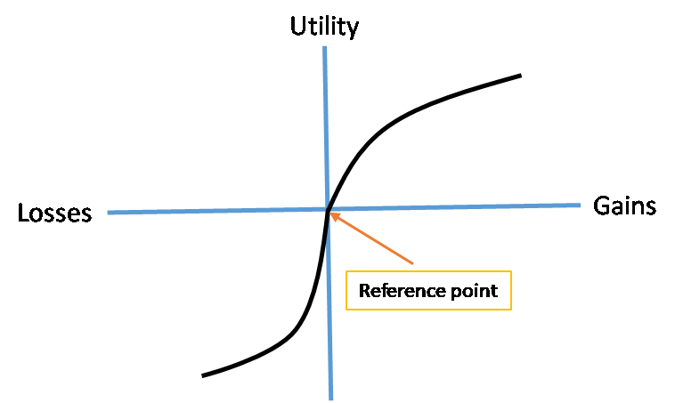
Begin by noticing that the “reference point” for the value function is not the individual’s initial wealth level.^[2] Rather it is the origin of the graph, here corresponding to $0. Next, as mentioned above, note that utility derived from gains, or a lottery’s winnings, is concave just as it is for our original utility function $u(w_i )$ . Thus, the value function similarly depicts diminishing sensitivity to gains. Finally, note that the individual’s disutility derived from a lottery’s losses is not only concave (thus depicting diminishing sensitivity to losses), but is also everywhere steeper, reflecting loss aversion.^[3] As you will see later in Section 4, reference dependence and loss aversion have played heavily in subsequent empirical research and choice infrastructure in the field of behavioral economics.^[4]

One immediate implication of the value function’s shape in Figure 4.1 is that it is always best for Homo sapiens to aggregate losses but segregate gains. As an example, suppose Homo sapiens Sally suffers two distinct losses in a single evening out on the town but also enjoys two distinct gains. The losses are (1) the $50 concert ticket she lost somewhere on the way to the theater, which she only realized was lost at the theater’s entrance; and (2) the extra $20 she had to pay to park closer to the theater that evening because she was running late. Her two gains from the evening were (1) the $20 bill she happened to find on the sidewalk out in front of the theater; and (2) the $25 bill at the restaurant that her friends paid for because they felt bad about Sally’s losses from earlier that evening.

According to the value function, Sally will experience less disutility from her losses if she thinks of them in the aggregate—as a single $70 loss—rather than two separate losses of $50 and $20. Because the value function is concave shaped in the loss region, the disutility corresponding to a $70 loss is less than the total disutility corresponding to separate losses of $50 and $20. Using similar reasoning, Sally will experience more utility from her gains if she thinks of them separately—as separate gains of $20 and $25—rather than as a single gain of $45. This is because of the value function’s concave shape defined over utility obtained from gains.

Thaler (1985) tested this implication of the value function and found that whether Homo sapiens choose to integrate losses and segregate gains depends upon how the losses and gains are framed to them in an experiment. This phenomenon is known as “hedonic framing.” Notwithstanding this experimental evidence, the implication’s lesson is clear: Homo sapiens would do well to aggregate multiple losses into a single loss and to keep multiple gains separated. As we will see below, this form of mind control is an example of what is known as “mental accounting.” Although behavioral economists generally believe that mental accounting leads to sub-optimal decision-making via distorting an individual’s allocation of wealth across the consumption of goods and services (c.f., Just, 2013), the value function implies that there are indeed situations where Homo sapiens can use mental accounting to their advantage.^[5]

Another closely related implication of the value function is what’s known as “hedonic editing.” This is a case where individuals who lose something that was recently gifted to them are better off considering the loss as an elimination of a gain (originally attained from the gift) rather than as an outright loss. This is due to the steeper slope of the value function defined over losses relative to its slope over gains. Thaler and Johnson (1990) tested this implication in laboratory experiments over different periods of time and found no clear, convincing evidence that Homo sapiens engage in hedonic editing.

As a point of reference (not a reference point per se), Cartwright (2014) proffers a simple functional form for Kahneman and Tversky’s (1979) value function depicted in Figure 4.1,

$v(x;r,\alpha,\beta,\lambda)={\Large \{ }\begin{matrix}(x-r)^\alpha \quad if \quad x \ge r \\-\lambda(r-x)^\beta \quad if \quad r>x \end{matrix}$

where $x$ represents the expected gain or loss experienced by an individual in relation to reference point $r$ , and $\alpha > 0$ , $\beta > 0$ , and $\lambda > 0$ represent the function’s additional parameters.^[6] When the individual experiences a gain, $x \ge r$ , the value function assigns a value of $(x-r)^\alpha >0$ to that gain. And when the individual experiences a loss, the function assigns a value of $-\lambda (r-x)^\beta <0$ . To depict the value function in Figure 4.1, we must further refine the parameter values in $v(x;r,\alpha ,\beta ,\lambda)$ . For those of you with strong enough math backgrounds, you will note that the depiction of Figure 4.1 requires $r=0$ , $0< \alpha <1$ , $0 < \beta < 1$ , and $\lambda > 1$ . The additional restrictions on $\alpha$ and $\beta$ ( i.e., $\alpha < 1$ and $\beta < 1$ ) ensure diminishing sensitivity to gains and losses, and $\lambda > 1$ ensures loss aversion ( $\lambda$ is commonly known as the “coefficient of loss aversion”). These restrictions are revisited below when we briefly explore an alternative theory of Homo sapiens choice behavior known as Regret Theory.

Using results from a laboratory experiment with their students, Tversky and Kahneman (1992) were able to estimate parameters $\alpha$ , $\beta$ , and $\lambda$ ; their median values being $\alpha = \beta$ = 0.88 and $\lambda$ = 2.25. Further, the authors estimate decision weights that are calculated subjectively (and subconsciously) by Homo sapiens to adjust the objective probabilities associated with the gains and losses of any given lottery (note from Chapter 3 that objective probabilities $p_g$ (for gain) and $p_l$ (for loss) could be used by Homo economicus to calculate the expected value, $x$ , of a given lottery as $x=p_gw_g+p_lw_l$ , where $w_g$ and $w_l$ are the values of the lottery’s gains and losses, respectively). Tversky and Kahneman (1992) estimated these decision weights, $\pi_i\left(p_i\right), \ i=g,l$ , using the nasty-looking formula,

$\pi_i (p_i)=\frac{p_i^{\gamma_i}}{{(p_i^{\gamma_i}+\left(1-p_i\right)^{\gamma_i})}^{1/\gamma_i}}$

where the median value for parameters $\gamma_i$ were estimated as $\gamma_g$ = 0.61 and $\gamma_l$ = 0.69. Thus, if the probabilities of gain and loss associated with a given lottery are $p_g$ = 0.6 and $p_l$ = 0.4, then using Tversky and Kahneman’s median values for $\gamma_g$ and $\gamma_l$ results in decision weights of $\pi_g$ = 0.47 and $\pi_l$ = 0.39. Thus, in relation to their corresponding objective probabilities, Homo sapiens’ subjective decision weights effectively reduce the lottery’s probabilities associated with both the gains and losses, with the magnitude of the reduction applied to the probability of gain being larger than that applied to the probability of loss.

By way of example, if the lottery’s gain is $w_g$ = $100 and loss is $w_l$ = -$105, then Homo economicus would calculate the lottery’s expected value as (0.6 x $100) – (0.4 x 105) = $18, while Homo sapiens would calculate the value as (0.47 x $100) – (0.39 x 105) = $6. Although our example here suggests that Tversky and Kahneman’s decision weights end up underweighting the objective probabilities of a lottery, we explain in Chapter 6 how the decision weights actually overweight improbable events (e.g., for a lottery with $p_g$ = 0.05 rather than 0.6, as in our example here).^[7]

Do reference dependence and loss aversion as embodied by value function $v\left(x;r,\alpha,\beta,\lambda\right)$ have implications for Homo sapiens’ indifference curve? In a word, yes. As Just (2013) shows, reference dependence and loss aversion imply the existence of an almost-imperceptible kink in an individual’s indifference curve at the reference point. To see this, consider Figure 4.2 below where bundle A represents the individual’s reference point. By the monotonicity property, we know that any move in the northeast direction from bundle A to a bundle including more of both goods 1 and 2 puts the individual on a higher indifference curve representing higher utility. To the contrary, any move to the southwest from bundle A to a bundle including less of both goods places the individual on a lower indifference curve representing lower utility. But what of moves to the northwest or southeast of bundle A?

Figure 4.2. Homo sapiens’ Kinked Indifference Curve

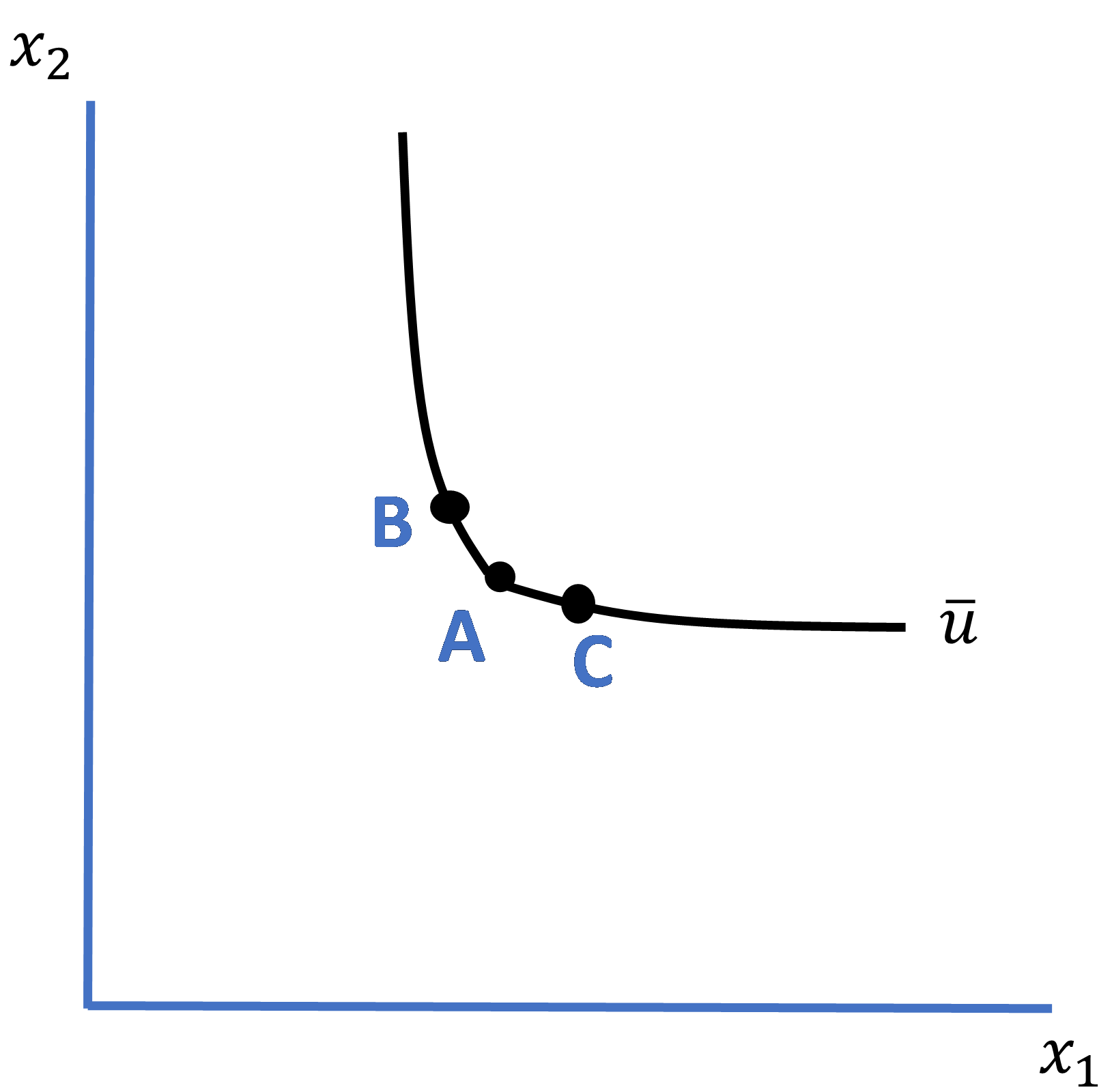
Begin by considering moves from bundle A northwest and southeast to new bundles B and C, respectively, along the indifference curve, where bundles B and C lie in what’s known as a “local neighborhood” of bundle A (i.e., very close to bundle A). Note that the amount of good 1 in new bundle B must have decreased relative to its amount in bundle A, and the amount of good 2 must have increased. This case is vice-versa for bundle C, where the amount of good 1 has increased and the amount of good 2 has decreased.

Now, because of Homo sapiens’ proclivity for loss aversion, which you will recall manifests itself in a value function exhibiting an everywhere steeper curve defined over losses than over gains, it must be the case that the increase in bundle B’s amount of good 2 is larger than its decrease in good 1. Otherwise, the individual would suffer a net loss in utility via loss aversion which, in turn, suggests that his utility would have to be represented by a lower (in the southwest direction) indifference curve rather than the one depicted by utility level $\bar{u}$ in the figure. By similar reasoning, it must be the case that bundle C’s increase in good 1 is larger than its decrease in good 2. Otherwise, the individual would again suffer a net loss in utility via loss aversion. Thus, pulling these arguments together, the slope of the indifference curve between bundles A and B in Figure 4.2 must be larger than the slope of the curve between bundles A and C. While the stylistic, smoothly convex indifference curve typifies the preferences of Homo economicus, the stylistic indifference curve attributable to Homo sapiens exhibits tiny kinks throughout.

Furthermore, Just (2013) shows that if we reconsider the indifference curves for Homo sapiens as being reference-dependent themselves, then our family of reference-dependent indifference curves can accommodate intersections, unlike for Homo economicus, for whom reference dependence is a non-issue. Loss aversion is not necessary to obtain this result.^[8]

To see what happens when an individual’s, say Jill’s, indifference curves depict reference dependence, consider Figure 4.3 below where $\bar{u}|_{R_1}$ represents the utility level over which Jill’s indifference curve is defined given reference bundle R1 and $\bar{u}|_{R_2}$ represents the utility level over which Jill’s indifference curve is defined given reference bundle R2 (a mouthful, I know, but hopefully you can see this).^[9]

Figure 4.3. Homo sapiens’ Reference-Dependent Indifference Curves

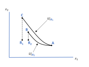
Now consider bundle A in relation to reference bundles R1 and R2. Note that because reference bundles R1 and R2 each include the same amount of good 2, Jill gives up the same amount of good 2 by moving from either of the reference bundles to bundle A. In contrast, the amount of good 1 Jill obtains by moving from reference bundle R1 to bundle A is greater than the amount Jill gains of good 1 by moving from reference bundle R2 to bundle A. Do you see that?

And now comes the fun part—consider the following thought experiment. Starting with reference bundle R1, suppose Jill switches to bundle A and then is posed the following questions:

“Jill, if you now had to sacrifice the increase in good 1 that you just obtained by switching from bundle R1 to bundle A, how much additional amount of good 2 would you require in order to retain utility level $\bar{u}|_{R_1}$ ? And if you instead started with reference bundle R2 and again had to sacrifice the increase in good 1 that you just obtained by switching from bundle R2 to bundle A, how much additional amount of good 2 would you require in order to retain utility level $\bar{u}|_{R_2}$ ?”

Since the amount of good 1 gained in the move to bundle A is larger relative to bundle R1 than to bundle R2, the corresponding amount of good 2 Jill would require to maintain utility level $\bar{u}|_{R_1}$ likewise exceeds the amount of good 2 required for Jill to maintain utility level $\bar{u}|_{R_2}$ (via an application of the Monotonicity Property). Thus, connecting the dots, so to speak, Jill’s reference-dependent indifference curve corresponding to reference bundle R1 (which includes points A and C) in Figure 4.3 is steeper than her curve corresponding to reference bundle R2 (which includes points A and B). Voila! The two indifference curves intersect at bundle A, which suggests a violation of the Transitivity Axiom from Chapter 3.

Again, because reference dependence is a non-issue for Homo economicus , reference-dependent indifference curves as drawn in Figure 4.3 are a non-starter for them. When it comes to indifference curves describing Homo economicus, we are restricted to drawing curves like those depicted in Figure 3.4.

Regret Theory**

As an alternative to Kahneman and Tversky’s Prospect Theory, Loomes and Sugden (1982 and 1987) propose what they have called Regret Theory; a theory with implications for both the expected utility theory ascribed to Homo economicus and Prospect Theory’s main constructs, in particular the causes of preference reversals (you will learn more about preference reversals in Chapter 5).

Regret Theory posits that an individual’s preferences for a given lottery depends explicitly upon the other “unchosen” lottery (i.e., the tradeoff the individual makes between the chosen and unchosen lotteries). As a point of reference, recall Homo economicus’ original utility function defined over wealth level $w$ , $u(w)$ , associated with a lottery ultimately chosen by the individual, say lottery $L$ . Similar to Prospect Theory, which extended utility function $u(w)$ to value function $v\left(x;r,\alpha,\beta,\lambda\right)$ , Regret Theory, in its most general form, extends Homo economicus’ utility function to Homo sapiens’ “Regret Theory Utility Function” $u\left(x,y\right)$ , where now the individual’s utility is simultaneously defined over levels $x$ from a chosen lottery, say lottery $L$ , and $y$ from the unchosen lottery $L^\prime$ (Just, 2013). While function $u\left(x,y\right)$ is still increasing in $x$ (as it is for Homo economicus), it is decreasing in $y$ . For example, if the two lotteries are such that the individual ultimately receives $5 from chosen lottery $L$ (i.e., $x$ = $5) when unchosen lottery $L^\prime$ would have yielded $1 ( $y$ = $1), he is happier than if $y$ would have instead yielded anything greater than $1 ( $y$ > $1). As long as $y<x$ , the individual “rejoices” with $u\left(x,y\right)>0$ . If instead $y>x$ , the individual experiences “regret” with $u\left(x,y\right)<0$ . At the threshold where $y$ = $x$ , $u\left(x,y\right)$ = 0. Regret Theory proposes that Homo sapiens maximize the expectation of $u\left(x,y\right)$ .

As Just (2013) explains, one version of the theory imposes symmetry on the individual’s utility levels associated with rejoicing and regret (called skew symmetry) as well as super-additivity on the individual’s utility function defined over regret (called regret aversion). Specifically, skew symmetry requires $u\left(x,y\right)=-u\left(y,x\right)$ along with $u\left(x,y\right)$ = 0 when $x$ = $y$ . Letting $z$ represent the outcome of another unchosen lottery, regret aversion requires $u\left(y,x\right)<u\left(y,z\right)+u\left(z,x\right)<0$ when the outcomes from the corresponding lotteries are $y>z>x$ (i.e., an individual regrets two small disappointments less than a single large one). With these properties in hand, Just (2013) goes on to show that Regret Theory can indeed justify preference reversals in the form of violations of the Transitivity Axiom—that is, to the extent that it accurately depicts the emotion of regret suffered by Homo sapiens, Regret Theory admits preference reversals, which are anathema to the rational-choice dictates of Homo economicus.

It should come as no surprise that Regret Theory Utility Function admits preference reversals. Similar to what we showed earlier in Figure 4.3, reference-dependent indifference curves intersect. The Regret Theory Utility Function formalizes reference dependence via explicitly including the outcome associated with the unchosen lottery, $y$ , as a variable in the function. Outcome $y$ in turn acts as the individual’s reference point.

Indeed, we can cast $u\left(x,y\right)$ directly in terms of value function $v\left(x;r,\alpha,\beta,\lambda\right)$ because of this correspondence between reference points $r$ from Prospect Theory and $y$ from Regret Theory—in effect $r$ = $y$ . Further, we can interpret skew symmetry as implying $\lambda$ = 1 and regret aversion as implying $\beta>1$ (as opposed to $\lambda$ = 1 and $0<\beta<1$ , respectively, for Prospect Theory according to Cartwright’s (2014) simple functional form for the value function). As a result, the value function depicted in Figure 4.1 is recast for Regret Theory as Figure 4.4.

Figure 4.4. Homo sapiens’ Value Function (Regret Theory)

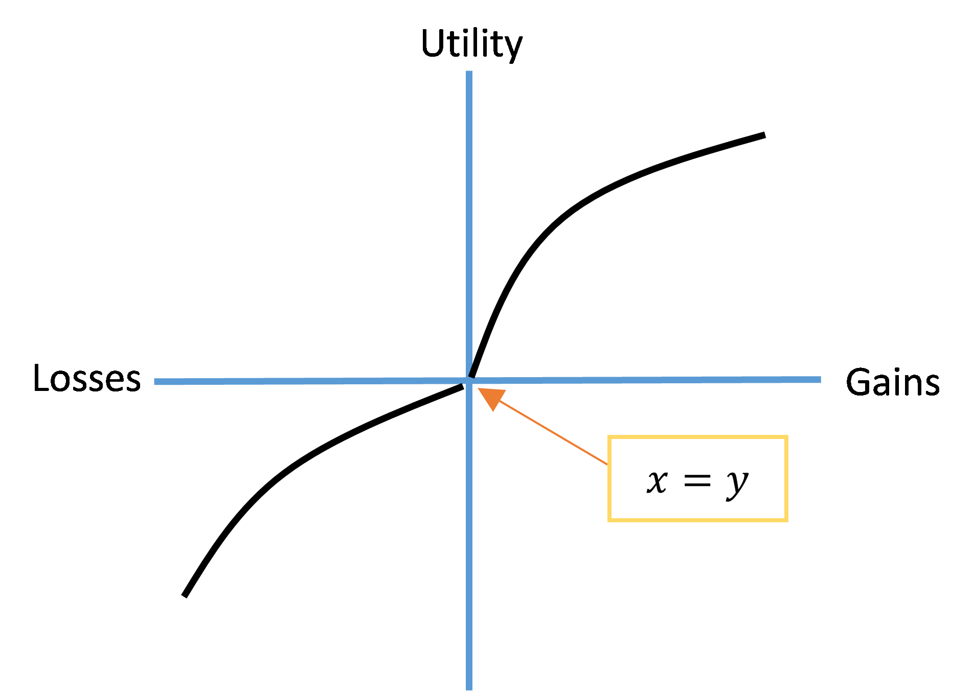
Note two things about the Regret Theory version of the value function in this figure. First, the portion of the curve defined over losses is convex-shaped rather than concave-shaped, as it is for the Prospect Theory version of the curve (recall Figure 4.1). Second, the portion of the curve defined over losses is not necessarily more steeply sloped than the portion defined over gains. This is because Regret Theory does not propound the notion of loss aversion.

Homo sapiens and Intertemporal Choice***

In Chapter 3 we learned that when confronted with an intertemporal choice problem, Homo economicus maintains stable preferences over consumption goods, adopts exponential time discounting, and as a result, exhibits stationarity in choice comparisons over time.^[10] As a result, Homo economicus makes time-consistent choices in terms of her consumption profile (and, by default, savings profile) over time. In other words, the consumption profile chosen by Homo economicus at the outset of her intertemporal decision problem does not change as she progresses from period to period and effectively re-solves her decision problem from each period forward. Clearly, from both theoretical and practical standpoints, any number of complications—embodied as relaxations of our model’s underlying assumptions—could lead to an appearance of time-inconsistent choices. Foremost among these assumptions are perfect foresight and the constancy of preferences, prices, and income, which were described in Chapter 3. However, to level the proverbial playing field of comparison between the intertemporal choice problems of Homo economicus and Homo sapiens, we retain these assumptions. The only assumption we dispense with is exponential time discounting and with it the condition of stationarity.

Based upon a simple laboratory experiment, Thaler (1981) found that when offered one apple today or two tomorrow, most subjects choose one today—an extra day is too long to wait to receive only one additional apple. However, if asked the same question about one apple a year from now or two apples one year and one day from now, the subjects’ preferences often reverse—they prefer to wait the extra day for the additional apple. After waiting a year, a day does not seem very long to wait to double consumption. Since the time interval between the choices is the same—one day in each case—this occurrence violates stationarity. Homo economicus would instead choose one apple today and one apple a year from now.

To capture this phenomenon—this violation of stationarity—among Homo sapiens, we replace the exponential time discounting practiced by Homo economicus with what’s come to be known as ”hyperbolic time discounting” (Ainslie, 1992).^[11] Recall from Chapter 3 that exponential time discounting is based upon constant discount factor $\delta$ , resulting in the set of discount factors over time,

$\delta\left(t\right)=\delta^t,\ t=0,\ldots,T$ ,

where time period $t=0$ corresponds to the initial period and $t=T$ represents the final period, which in Chapter 3 was period 3, but which, in theory, could extend to $T=\infty$ . Following Just (2014), hyperbolic discounting leads to a corresponding set of discount factors over time defined by,

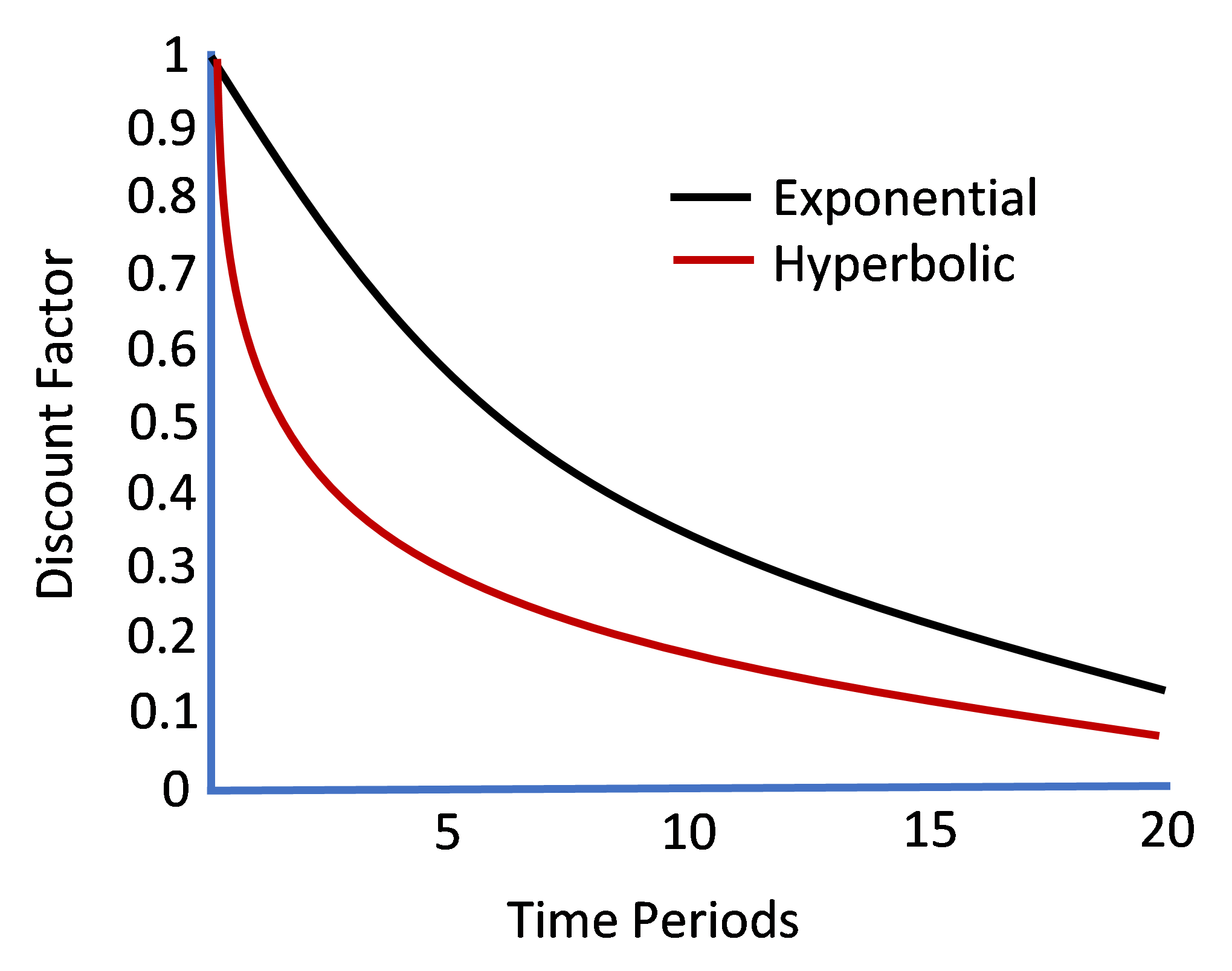
$h\left(t\right)=\left(1+\alpha t\right)^{-\left(\sfrac{\beta}{\alpha}\right)},\ t=0,\ldots,T$ ,

where scalars $\alpha > 0$ and $\beta > 0$ . Both the exponential and hyperbolic discounting functions are depicted in Figure 4.5 for the case of $\alpha$ = $\beta$ = 1 and $\delta<1$ . Compared with the exponential discounting function, the hyperbolic discount factor declines more quickly over the first few time periods. Thus, an individual who abides by hyperbolic discounting values near-term future consumption much less than someone who abides by exponential discounting. The hyperbolic discounting function also declines very slowly over the latter periods relative to the exponential discounting function. Thus, an individual who abides by hyperbolic time discounting is more willing to delay consumption in the distant future than in the near future relative to an individual who discounts exponentially. In terms of Thaler’s (1981) apple experiment, these discounting functions suggest that while subjects abiding by exponential and hyperbolic discounting might both prefer an apple today rather than two apples tomorrow, subjects using hyperbolic discounting may end up preferring two apples a year and a day from now than one apple one year from now.^[12], ^[13]

Figure 4.5. Hyperbolic vs. Exponential Time Discounting

Hence, Homo sapiens—who, as Thaler (1981) proposes, tend to adopt hyperbolic time discounting—do not display intertemporal preferences that adhere to stationarity. To see this formally, we borrow the notation from Chapter 3 for the individual’s three-period choice decision and assume that $\alpha$ = $\beta$ = 1 in hyperbolic discounting function $h\left(t\right)=\left(1+\alpha t\right)^{-\left(\sfrac{\beta}{\alpha}\right)}$ , resulting in,

$\begin{matrix}Max\\\left\{x_1,x_2,x_3\right\}\\\end{matrix}\ \ u\left(x_1\right)+\frac{u\left(x_2\right)}{2}+\frac{u\left(x_3\right)}{3}$ ,

subject to,

$W=\left(p_1\cdot x_1\right)+\left(p_2\cdot x_2\right)+\left(p_3\cdot x_3\right)$ ,

where, for discounting purposes, we treat period 1 as equaling zero in the discounting function, and periods 2 and 3 as equaling one and two, respectively. Again, for those of you familiar with calculus, in particular solving constrained optimization problems, recall that you can write this problem in its Lagrangian form as,

$\mathcal{L}=u\left(x_1\right)+\frac{u\left(x_2\right)}{2}+\frac{u\left(x_3\right)}{3}$

where $\lambda>0$ represents the problem’s Lagrangian multiplier, and again for simplicity, we have normalized all prices to one (i.e., $p_1=p_2=p_3=1$ ). Obtaining the associated system of first-order conditions for this problem results in $u^\prime\left(x_1\right)=u^\prime\left(x_2\right)/2=u^\prime\left(x_3\right)/3=\lambda$ , where $u^\prime\left(\cdot\right)$ denotes the individual’s marginal utility function. Similar to Homo economicus’ choice problem from Chapter 3, this string of equalities indicates that discounted marginal utility levels are equated across time. Given our underlying assumption of diminishing marginal utility, the string of equalities again implies $x_1^\ast>x_2^\ast>x_3^\ast$ , i.e., the individual optimally consumes more in the first period than in the second, and more in the second period than the third.

To test Homo sapiens for stationarity, we follow the same approach used to test Homo economicus in Chapter 3:

Suppose a member of Homo sapiens chooses to consume the same base amount $x$ in each period and let two different increments to consumption be denoted as $i_1$ and $i_2$ . Stationarity implies that if $u\left(x+i_1\right)>u\left(x+i_2\right)/2$ , where $u\left(x+i_1\right)$ represents the corresponding utility level in period 1 and $u\left(x+i_2\right)/2$ represents discounted utility level in period 2, then $u\left(x+i_1\right)/2>u\left(x+i_2\right)/3$ by exactly the same amount as $u\left(x+i_1\right)>u\left(x+i_2\right)/2$ , where $u\left(x+i_2\right)/3$ represents discounted utility level in period 3. However, unlike what was shown for Homo economicus under exponential time discounting in Chapter 3, here we see that for Homo sapiens under hyperbolic time discounting, $\left(u\left(x+i_1\right)/2-u\left(x+i_2\right)/3\right)$ does not equal $\left(u\left(x+i_1\right)-u\left(x+i_2\right)/2\right)$ . Hence, Homo sapiens’ preferences are not stationary through time.

Lastly, to see why Homo sapiens’ preferences are potentially time inconsistent with hyperbolic discounting, we follow the same approach as was used to test Homo economicus for time consistency.^[14] Given that he has chosen $x_1^\ast,\ x_2^\ast$ , and $x_3^\ast$ at the outset for any given set of $\delta$ , $W$ , and prices $p_1,p_2$ , and $p_3$ , if after having consumed at level $x_1^\ast$ in period 1, the individual decides to re-solve his decision problem from that point forward (i.e., now starting in period 2), he effectively solves,

$\begin{matrix}Max\\\left\{x_2,x_3\right\}\\\end{matrix}\ \ u\left(x_2\right)+\frac{u\left(x_3\right)}{2}$ ,

subject to,

$W=2w=\left(p_2\cdot x_2\right)+\left(p_3\cdot x_3\right)$ ,

which does not necessarily result in the same $x_2^\ast$ and $x_3^\ast$ as before. To see this result, first pull $u^\prime\left(x_2\right)/2=u^\prime\left(x_3\right)/3$ from the string of three equalities derived from the individual’s original decision problem (i.e., $u^\prime\left(x_1\right)=u^\prime\left(x_2\right)/2=u^\prime\left(x_3\right)/3$ ). Next, note that $u^\prime\left(x_2\right)/2=u^\prime\left(x_3\right)/3$ is not the same equality resulting from the first-order conditions for this two-period problem, which is $u^\prime\left(x_2\right)=u^\prime\left(x_3\right)/2$ . Therefore, given that nothing else has changed in this problem (i.e., the values for $\delta$ , $w$ , and $p_1,p_2$ , and $p_3$ are the same, as is the functional form of $u\left(\cdot\right)$ ), the values for $x_2$ and $x_3$ that solve Homo sapiens’ two-period problem (here denoted as $x_2^{\ast\ast}$ and $x_3^{\ast\ast}$ , respectively) are not the same as the values for $x_2^\ast$ and $x_3^\ast$ that have solved his original three-period problem, specifically, $x_2^{\ast\ast}>\ x_2^\ast$ and $x_3^{\ast\ast}<\ x_3^\ast$ . Thus, Homo sapiens’ consumption profile is potentially time-inconsistent.

To see this last result, we first rewrite the equality from the individual’s three-period problem, $u^\prime\left(x_2\right)/2=u^\prime\left(x_3\right)/3$ , as $u^\prime\left(x_2\right)={2u}^\prime\left(x_3\right)/3$ and then compare directly with the equality from the individual’s two-period problem, $u^\prime\left(x_2\right)=u^\prime\left(x_3\right)/2$ . Because the right-hand side of the former equality (i.e., ${2u}^\prime\left(x_3\right)/3$ ) is larger than the right-hand side of the latter equality (i.e., $u^\prime\left(x_3\right)/2$ ), if we take the $x_2$ and $x_3$ that solve the first equality (i.e., $x_2^\ast$ and $x_3^\ast$ ) and plug these values into the second equality, then that equality no longer holds, in specific $u^\prime\left(x_2^\ast\right)>u^\prime\left(x_3^\ast\right)/2$ . Given the assumption of diminishing marginal utility (i.e., that function $u^\prime\left(\cdot\right)$ decreases in $x$ ), and that annual income levels and all prices are fixed and constant, it therefore must be the case that $x_2^{\ast\ast}>\ x_2^\ast$ and $x_3^{\ast\ast}<\ x_3^\ast$ in order restore the equality.

You should note that this potential time-inconsistency result suggests that hyperbolic discounting provides a theoretical justification for why Homo sapiens are prone to procrastinate. If we think of the consumption good as embodying the value obtained from the feeling of relief that comes with putting forth the necessary effort to finish a task, then $x_2^{\ast\ast}>\ x_2^\ast$ implies that the need to feel relief becomes more urgent (or valuable) by the time the individual reaches the second period. In other words, with hyperbolic discounting Homo sapiens undervalue the feeling of relief at the outset. As time goes by though (i.e., as he reaches the second period), Homo sapiens overcompensates his effort to obtain the feeling of relief. Sound like a recipe for procrastination? At the very least, hyperbolic time discounting is one of the recipe’s main ingredients.

Key Takeaways on Homo sapiens**

We conclude this chapter by revisiting the two central contributions of Kahneman and Tversky’s (1979) Prospect Theory discussed earlier: reference dependence and loss aversion. We also introduce a new effect known as the Endowment Effect, which is a special case of the Anchoring Effect introduced in Chapter 1 and is also an expression of Status Quo Bias introduced in Chapter 2. As we will see in Chapter 5 and later in Section 4, the Endowment Effect has been the focus of several experiments.

Earlier, we relied upon a graphical representation of the value function to depict how the presence of reference dependence and loss aversion impelled a departure from the rational-choice model’s conception of the expected utility form—the form used to represent Homo economicus’ preferences over uncertain wealth and attendant risks. Here, following Tversky and Kahneman (1991), we depict all three idiosyncrasies in a single, indifference-curve framework.^[15]

In Figure 4.6 below, the two “commodities” measured on the horizontal and vertical axes are, respectively, the number of vacation days and the annual income accruing to our exemplary individual, Tammy. Initially, Tammy is located at Bundle 1, earning $100,000 and taking 14 vacation days per year, and as a result, attaining ${\bar{u}}_1$ utils of happiness.

Figure 4.6. Reference Dependence, Loss Aversion, and the Endowment Effect

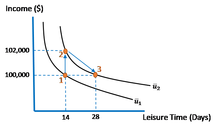
Suppose Tammy is now given a raise (finally!) of $2,000 per year. She moves to Bundle 2, attaining the higher ${\bar{u}}_2$ utils of happiness. A month later, out of the blue, her boss asks Tammy if she would be willing to forfeit the $2,000 raise and instead take an extra 14 days of vacation time each year. If she accepts her boss’ offer, she would therefore move to Bundle 3. Because she is on the same indifference curve with Bundle 3 as she is with Bundle 2, Tammy would still attain ${\bar{u}}_2$ utils of happiness.

To the extent that Tammy behaves more like a Homo economicus than Homo sapiens, what we would expect Tammy to do—hang on to her raise and forgo the extra 14 days of vacation time (i.e., remain at Bundle 2), or forfeit her raise and nab the extra vacation time (i.e., move to Bundle 3)? As a member of Homo economicus, Tammy would not suffer from reference dependence or loss aversion in moving from Bundle 2 to Bundle 3. And in this case, because her utility level remains constant at ${\bar{u}}_2$ , neither would she exhibit an endowment effect. An Endowment Effect occurs when an individual perceives herself as better off in the status quo (e.g., at bundle 2) even when her utility level in the status quo is no higher than in a different state of the world (e.g., bundle 3). As a result, Tammy would be no worse off flipping a fair coin and letting the outcome of the coin flip determine her choice (e.g., “heads I stick with Bundle 2, tails I change to Bundle 3”).

This would not be so if Tammy is a member of Homo sapiens. As a Homo sapiens, we would expect her to be partially governed by all three idiosyncrasies. Regarding reference dependence, consider the fact that Tammy has only enjoyed her raise in pay for one month. This bump in her income is therefore likely to be fresh in her mind. To the extent that this is the case, it could be that in the interim of having received the pay raise and being given the opportunity of choosing Bundle 3, her indifference curve associated with utility level ${\bar{u}}_2$ has actually gotten flatter in the region between Bundles 2 and 3 (with Bundle 2 serving as a pivot point), and thus, choosing Bundle 3 would now result in her attaining a utility level less than ${\bar{u}}_2$ (sketch this possibility in Figure 4.6 and see for yourself). Tammy therefore would not flip a coin. She would turn down her boss’ offer and stick with Bundle 2.

Alternatively, it could be that Tammy’s reference point for this decision is stuck at Bundle 1. One month hasn’t really been long enough for her to learn to enjoy the added utility that she will eventually obtain from the pay raise. So, in her mind, Tammy actually compares Bundles 1 and 3, not Bundles 2 and 3. In this case, Tammy will accept the boss’s offer and switch to Bundle 3. As far as Tammy in concerned, she has gained ${\bar{u}}_2$ – ${\bar{u}}_1$ utils of happiness in making the switch.

Either way, therefore, reference dependence nuances Tammy’s decision when she thinks more like Homo sapiens than Homo economicus.

The story is less ambiguous regarding loss aversion. To the extent that Tammy suffers from loss aversion, she will interpret the certain loss of her $2,000 pay raise as inducing a greater loss in utility than the potential gain in happiness that will come with 14 more vacation days. Hence, loss aversion points Tammy toward rejecting her boss’ offer and sticking with Bundle 2 in Figure 4.6.

Finally, let’s consider the possibility of Tammy experiencing an Endowment Effect as a member of Homo economicus. Because the move from Bundle 2 to Bundle 3 does not change her utility level, we would not expect Tammy, as Homo economicus, to suffer from an endowment effect (i.e., to necessarily choose Bundle 2 over Bundle 3). However, as a member of Homo sapiens, the Endowment Effect is potentially alive and well. Tammy could be covetous of her recent pay raise, and therefore would not be indifferent between Bundles 2 and 3. She would be more likely to stick with Bundle 2.

Tallying up the score in Figure 4.6 (and remembering that Tammy is, after all, a member of Homo sapiens), it seems that, contrary to what rational-choice theory would suggest, the three idiosyncrasies—reference dependence, loss aversion, and the Endowment Effect—point Tammy toward rejecting her boss’ added-vacation offer and sticking with Bundle 2. At the very least, we should not be as confident in concluding that she will base her decision on a flip of a coin, as we would if she were miraculously a member of Homo economicus instead.

We conclude with a few quick thought experiments before taking a headlong dive into the famous laboratory experiments that have propelled the field of behavioral economics into the limelight.

Consider the following thought experiment:

Today, Sally and Sam each have wealth worth $5 million. Yesterday, Sally had wealth worth $1 million and Sam had wealth worth $9 million. Are Sally and Sam equally happy today?

If you answered “no,” then you believe that Sally and Sam’s utilities are each reference dependent. By default, Homo economicus would answer “yes” because what matters in the rational choice model is total wealth (which is currently at the same level for Sally and Sam), not actual gains and losses.

Now consider this thought experiment:

Which lottery do you prefer?

A 85% chance to lose $1000 and 15% chance to lose nothing
B certain loss of $800

If you chose lottery A, then you are a “risk seeker” and exhibit loss aversion. Homo economicus would have done the math, and since her expected loss from lottery A is a larger number than the certain loss from lottery B, she would have chosen lottery B.

Study Questions

Note: Questions marked with a “†” are adopted from Just (2013), and those marked with a “‡” are adopted from Cartwright (2014).

^† Suppose Uncle Joe’s preferences can be depicted as a value function like that drawn in Figure 4.1. Last night Joe experienced both a gain and a loss. The gain was paying $25 less than he had expected for his dinner date with Auntie Jill. The loss was finding a $25 parking ticket waiting for him underneath his car’s wiper blade when he and Jill returned to the car following the meal. Would it be best, in terms of his overall utility level, if Joe segregated the gain from the loss or integrated the two? Explain.
Suppose an individual’s value function is depicted in the figure below. Which properties of Prospect Theory is this individual violating?
^‡ Suppose someone’s willingness-to-pay for a good is $10, and their reference point is $20. If the good is priced at $13, will they buy it? What does your answer say about sales and “bargain buys”?
Is the Monotonicity Property necessary for an individual’s reference-dependent indifference curves to cross? Why?
^† Suppose Akira has two sources of income. Anticipated income (e.g., accrued from her regular weekly paycheck), $w_1$ , is spent on healthy food, $x_1$ , and clothing, $x_2$ . Unanticipated income (e.g., inherited wealth), $w_2$ , is spent on what Akira considers to be a luxury good, $x_3$ . Suppose Akira’s value function is given by $v\left(x_1,x_2,x_3\right)=\left(x_1x_2x_3\right)^\frac{1}{3}$ , so that the marginal utilities associated with goods 1, 2, and 3, respectively, are given by ${MU}_1=\frac{1}{3}x_1^{-\frac{2}{3}}\left(x_2x_3\right)^\frac{1}{3}$ , ${MU}_2=\frac{1}{3}x_2^{-\frac{2}{3}}\left(x_1x_3\right)^\frac{1}{3}$ , and ${MU}_3=\frac{1}{3}x_3^{-\frac{2}{3}}\left(x_1x_2\right)^\frac{1}{3}$ . Suppose $w_1$ = $8 and $w_2$ = $2, and that corresponding per-unit prices for goods 1, 2, and 3 are given by $p_1=p_2$ = $1 and $p_3$ = $2, respectively. It can be shown that Akira’s optimal demands for goods 1, 2, and 3 are values 4, 4, and 1, respectively. To see this, we set the marginal utilities of consumption per dollar equal across $x_1$ and $x_2$ and then impose the condition(s) that the cost of all goods in the budget associated with the anticipated and unanticipated incomes are equal to their respective budget constraints. Hence, from the budget constraints for anticipated and unanticipated income, respectively, we set $x_1+x_2$ = 8 and $2=2x_3\Longrightarrow x_3=1$ . Setting $\frac{{MU}_1}{p_1}=\frac{{MU}_2}{p_2}\Longrightarrow x_1=x_2$ , which, given $x_1+x_2$ = 8, implies $x_1=x_2=4$ . (a) Suppose Akira receives an extra $4 in anticipated income, and thus $w_1$ = $12 and $w_2$ = $2. How does Akira’s demand for goods 1, 2, and 3 change? (b) Alternatively, suppose Akira receives the extra $4 as unanticipated income, and thus $w_1$ = $8 and $w_2$ = $6. How does Akira’s demand change now? Hint for parts (a) and (b): Use the same approach as was shown above to answer these two questions. (c) In relation to parts (a) and (b), could Akira make herself better off by not doing mental accounting (i.e., by not compartmentalizing the entire $4 increase into either anticipated or unanticipated income) and instead combine the two accounts into a single total income account and allocate the $4 increase in income to total income? Hint for part (c): Note that total income becomes $14, and the corresponding budget constraint is $14=x_1+x_2+2x_3$ . Again, noting that $\frac{{MU}_1}{p_1}=\frac{{MU}_2}{p_2}$ , and now $\frac{{MU}_1}{p_1}=\frac{{MU}_3}{p_3}$ as well, leads to the answer.
^‡ Suppose Anna owns her own house and house prices in the market increase. Should Anna spend more money on everyday living expenses? Suppose Anna also has money invested in the stock market and stock prices decrease. Should Anna spend less money on everyday living expenses? Explain.
^†Consider the Regret Theory Utility Function given by $u(x,y)={\Large \{ }\begin{matrix}(x-y)^2 \quad if \quad x \ge y \\-(y-x)^2 \quad if \quad y>x \end{matrix}$ . Plot the implied indifference curves for $u(x,y)$ = 1 and $u(x,y)$ = -1. Explain how these curves can be used to denote a preference reversal.
Explain why reference dependence in the context of Regret Theory can lead to the intersection of the reference-dependent indifference curves and thus a preference reversal.
Referring to the three-period hyperbolic time discounting problem discussed in this chapter, show that stationarity does not hold for utility function $u\left(x\right)=\ln{x}$ . Hint: Assume $\alpha$ = $\beta$ = 1. To show this result, you must then choose increments $i_1$ and $i_2$ such that $\ln{\left(x+\ i_1\right)>\frac{ln\left(x+\ i_2\right)}{2}}$ , and proceed from there.
^‡ Referring to the lotteries listed below, explain what Prospect Theory suggests Henrietta the Homo sapiens will choose to do vis-à-vis Lottery A vs. Lotteries B – F, respectively. Lottery A: Win $0 for certain. Lottery B: Lose $100 with probability of 0.5, win $105 otherwise. Lottery C: Lose $100 with probability of 0.5, win $125 otherwise. Lottery D: Lose $100 with probability of 0.5, win $200 otherwise. Lottery E: Lose $225 with probability 0.5, win $375 otherwise. Lottery F: Lose $600 with probability 0.5, win $36 million otherwise.
^† Harper is spending a three-day weekend at her beach property. Upon arrival, she purchases a quart of ice cream and must divide consumption of the quart over each of the three days. Her instantaneous utility of ice cream consumption is given by $u\left(x\right)=\sqrt x$ , where $x$ is measured in quarts, so that the instantaneous marginal utility is given by $u^\prime\left(x\right)=\frac{1}{2\sqrt x}$ . (a) Suppose Harper discounts future consumption of ice cream using exponential time discounting with a daily discount factor $\delta$ = 0.8. (a) Solve for Harper’s optimal consumption profile over the course of the three days by finding the daily proportions of the quart of ice cream that both equate the discounted marginal utilities of consumption across the three days, and sum to 1. (b) Now suppose that Harper discounts future utility according to hyperbolic time discounting, with $\alpha=\beta=1$ . Describe the optimal consumption profile starting from the first day of the weekend. How will the consumption plan change on day two?
^‡ Suppose Henrietta the Homo sapiens is prone to experience regret when it comes to choosing between different lotteries. She faces the following three lotteries: Lottery A: Win $5 for certain. Lottery B: Win $10 with probability of 0.4, win $3 with probability of 0.6. Lottery C: Win $7.50 with probability of 0.7, win $1 with probability of 0.3. Given what you know about Regret Theory, how might you explain Henrietta’s choices when comparing Lotteries A and B, B and C, and A and C, respectively?
What condition typically exhibited by Homo sapiens do businesses attempt to exploit when they advertise that “supplies won’t last long”?
^‡ Is it better to be an employee in a firm where you earn $50,000 per year and the average salary is $80,000 or in a firm where you earn $45,000 and the average salary is $30,000.
Why don’t the reference-dependent indifference curves $\bar{u}|_{R_1}$ and $\bar{u}|_{R_2}$ in Figure 4.3 extend to the southeast of Bundle A?

Media Attributions

Figure 4.3 v2

Remember our discussion about Jumping to Conclusions earlier in the book? ↵
Reference point is sometimes referred to as an anchor or saliency point. ↵
The ratio of the slopes of the loss and gain portions of the value function measured near the function’s origin is a formal measure of loss aversion. Empirical estimates of loss aversion are typically close to a value of two, meaning that the disutility associated with an incremental loss is twice as great as the utility associated with an incremental gain of the same magnitude (Tversky and Kahneman, 1991, and Kahneman et al., 1990). ↵
To whet your appetite, Odean (1998) used transaction data for 10,000 customers of a discount brokerage firm to examine how loss aversion might manifest itself in the trading decisions made by small-time investors in the stock market. He found that investors were much more likely to sell investments that had increased rather than decreased in value. This tendency to realize gains and avoid realizing losses (i.e., being averse to loss) is known as the Disposition Effect. ↵
Interestingly, purchasing goods and services with a credit card and paying off the balance at the end of each billing period is a convenient way for individuals to aggregate losses (you pay for all the goods purchased that period in one, painful lump-sum) and segregate gains (you enjoy your purchases as you make them). ↵
It is common notational practice to list a function’s parameters to the right of the semi-colon and the variable over which the function is defined to the left of the semi-colon within the parenthesis. ↵
A homework problem asks you to calculate the decision weight $\pi_g$ associated with $p_g$ = 0.05 using the above decision-weight formula. ↵
As we will discuss, however, the family of reference-dependent indifference curves cannot be drawn to simultaneously abide by the Transitivity Axiom and Monotonicity Property. The family of curves continues to abide by monotonicity but not transitivity, and in this respect, suggests that Homo sapiens can indeed exhibit preference reversals (since preference reversals are an implication of violating Transitivity). We wait until later in this section—after we have explored what’s known as the Endowment Effect—to couch the implications of reference dependence, loss aversion, and the endowment effect directly into Homo economicus’ family of non-reference-dependent indifference curves. ↵
Because they are reference-dependent indifference curves rather than non-reference-dependent, the curves in this figure do not exhibit a kink as they did in the previous figure. ↵
Recall that stationarity means that preferences for any increments of consumption in two different time periods depends upon the interval of time that passes between the two time periods (e.g., between periods 1 and 2), and not the specific points in time when the two respective increments could be consumed (e.g., periods 2 and 3). ↵
Laibson (1997) proposed a more tractable version of hyperbolic discounting that eventually became known as "quasi-hyperbolic discounting." As Cartwright (2014) explains, quasi-hyperbolic discounting can fully account for time-inconsistent behavior in Homo sapiens. ↵
Recall that if an individual abiding by exponential discounting prefers an apple today rather than two apples tomorrow, she will also prefer an apple a year from now more than two apples a year and a day from now. ↵
See Benzion et al. (1989) for a classic laboratory experiment designed to infer individuals’ time discounting regimes from choice scenarios involving (1) the postponement of a payment due (i.e., debt) until a later point in time, (2) postponement of a payment receipt (i.e., credit) until a later point in time, (3) expedition of a debt due in a future period to the current period, and (4) expedition of a credit expected in the future to the current period. ↵
As Cartwright (2014) explains, quasi-hyperbolic discounting, not hyperbolic discounting, is necessary to (theoretically) account for time-inconsistent behavior among Homo sapiens. It is for this reason that we stress “potentially” time inconsistent in this sentence. ↵
Kahneman et al. (1991) provide a nice synopsis of these key aspects of Prospect Theory. ↵

License

Icon for the Creative Commons Attribution 4.0 International License