The Rationality of <em>Homo economicus</em>

Arthur J. Caplan

3 The Rationality of Homo economicus

Principal Rationality Axioms*

Completeness Axiom

Suppose Homo economicus faces two lotteries, which we will denote as lotteries $L$ and $L^\prime$ , where both lotteries are taken from what is known as the space of available lotteries $\mathcal{L}$ . Then, it must be the case that either $L\succsim L^\prime$ , $L\precsim L^\prime$ , or $L\sim L^\prime$ . What the previous sentence says is that Homo economicus either likes lottery $L$ at least as much as lottery $L^\prime$ (i.e., $L\succsim L^\prime$ ), likes lottery $L^\prime$ at least as much as lottery $L$ (i.e., $L\precsim L^\prime$ ), or is indifferent between the two lotteries (i.e., $L\sim L^\prime$ ). This is known as the Completeness Axiom. For future reference, we will use the equivalent terminology “weakly preferred to” rather than “likes at least as much” when referring to the preference relation $\succsim$ .

Transitivity Axiom

Given any third lottery $L^{\prime\prime}$ taken from the space of available lotteries $\mathcal{L}$ , if $L\succsim L^\prime$ and $L^\prime\succsim L^{\prime\prime}$ , then $L\succsim L^{\prime\prime}$ . In other words, Homo economicus would never fall victim to a “preference reversal,” whereby she makes choices that contradict her stated preference ranking. This is known as the Transitivity Axiom.

So that we are clear on what a lottery is, here is an example of three possible lotteries $L$ , $L^\prime$ , and $L^{\prime\prime}$ .

As a final note, it is worth pointing out that the Principal Rationality Axioms imply the existence of what’s known as a utility function representing an individual’s preferences over lottery space $\mathcal{L}$ , specifically, $U:\mathcal{L}\rightarrow R$ such that $L\succsim L^\prime\Longleftrightarrow U\left(L\right)\geq U\left(L^\prime\right)$ . Let’s unpack this mathematical statement. The first part of the statement (i.e., $U:\mathcal{L}\rightarrow R$ ) says that utility function $U$ magically translates an individual’s preferences for the different lotteries that make up lottery space $\mathcal{L}$ into real numbers. The real numbers, by the way, are measured in what’s known as “utils,” or units of happiness. For example, if $U\left(L\right)$ = 100.3, then the individual facing lottery $L$ gets 100.3 units of happiness just from the opportunity of being able to play the lottery.

The second part of the statement (i.e., $L\succsim L^\prime\Longleftrightarrow U\left(L\right)\geq U\left(L^\prime\right)$ ) says that the statement “lottery $L$ is weakly preferred to lottery $L^\prime$ ” (i.e., $L\succsim L^\prime$ ) is equivalent to the statement “the utility level obtained from lottery $L$ is no less than the utility level obtained from lottery $L^\prime$ ” (i.e., $U\left(L\right)\geq U\left(L^\prime\right)$ ).

Additional Rationality Axioms*

Dominance Axiom

If $L\succsim L^\prime$ in all respects (i.e., $L$ ’s expected win outcomes are larger than $L^\prime$ ’s, and $L$ ’s expected loss outcomes are lower), then $L\succ L^\prime$ . To see what we mean by “expected win” and “expected loss” outcomes, refer to the example lotteries above in the discussion of the Transitivity Axiom. Lottery $L$ ’s expected win and expected loss outcomes, respectively, are $120 (0.6 x $200) and $40 (0.4 x $100), while lottery $L^\prime$ ’s are $50 (0.5 x $100) and $35 (0.5 x $70). The final part of this axiom’s statement, $L\succ L^\prime$ , states that lottery $L$ is “strictly” preferred to lottery $L^\prime$ . An equivalent way to say “strictly preferred to” is to say “likes more than.” This is known as the Dominance Axiom.

Again referring to the example above, is $L\succ L^\prime$ by the Dominance Axiom? The answer is “no.” Although lottery $L$ ’s expected win of $120 is larger than lottery $L^\prime$ ’s expected win of $50, $L$ ’s expected loss of $40 is also larger than $L^\prime$ ’s expected loss of $35. If lottery $L$ ’s expected loss had instead been some amount less than $35, we could have concluded that $L\succ L^\prime$ by the Dominance Axiom.

Invariance Axiom

If an individual’s preference ordering of different lotteries does not depend on how the lotteries are described, then the individual’s preferences satisfies the Invariance Axiom. We do not have a mathematical expression for this axiom. But there will be plenty of examples as we explore the seminal experiments conducted by Kahneman and Tversky, experiments that motivated their famous theories in behavioral economics. We will be learning about these theories later in this section of the textbook.

Sure-Thing Principle

If $L\succsim L^\prime$ in any possible known state of the world, then $L\succsim L^\prime$ even when the state of the world is unknown. This is known as the Sure-Thing Principle. Similar to the Invariance Axiom, we do not have a mathematical expression to contend with. We will soon see an example.

The Sure-Thing Principle implies that an individual does not need to consider uncertainties when making a decision if the individual deems the uncertainties to be irrelevant. For example, if an investor has decided to purchase a company’s stock regardless of its upcoming earnings report, then it makes no sense for the investor to worry about whether the company will ultimately report a profit or a loss. His preference for the company’s stock is unaffected by the uncertainty surrounding its reported profit level.

Independence Axiom

An individual’s preferences defined over lottery space $\mathcal{L}$ satisfies the Independence Axiom if for any three lotteries $L,L^\prime$ , and $\ L^{\prime\prime}$ , and some constant $\alpha$ that lies between 0 and 1 (non-inclusive of 0 and 1), we have,

$L\succsim L^\prime\Longleftrightarrow\alpha L+\left(1-\alpha\right)L^{\prime\prime}\succsim\alpha L^\prime+\left(1-\alpha\right)L^{\prime\prime}$ .

This last part of the axiom is a bit ugly. So let’s look at an example.

So that we are clear about how the various probabilities for lottery $\alpha L+\left(1-\alpha\right)L^{\prime\prime}$ are derived, note that because lottery $L$ includes the chance to win $200 and lottery $L^{\prime\prime}$ does not, we end up with a 36% (0.6 x 60%) chance of winning the $200. Similar logic is used for calculating the 22% chance of winning $20 (0.4 x 55%), the 24% chance of losing $100 (0.6 x 40%), and the 18% chance of losing $20 (0.4 x 45%). The same method applies to calculating the probabilities for lottery $\alpha L^\prime+\left(1-\alpha\right)L^{\prime\prime}$ .

Thus, in adherence to the Independence Axiom, if, say, an individual weakly prefers lottery $L$ to lottery $L^\prime$ , then that individual will also weakly prefer lottery $\alpha L+\left(1-\alpha\right)L^{\prime\prime}$ to lottery $\alpha L^\prime+\left(1-\alpha\right)L^{\prime\prime}$ . By the looks of our example, the comparison between lottery $\alpha L+\left(1-\alpha\right)L^{\prime\prime}$ and lottery $\alpha L^\prime+\left(1-\alpha\right)L^{\prime\prime}$ is likely to be difficult for Homo sapiens, who would thus be prone to violate this axiom. Hats off to Homo economicus for not violating the Independence Axiom.

Substitution Axiom

An individual’s preferences defined over lottery space $\mathcal{L}$ satisfies the Substitution Axiom if, for any two lotteries $L$ and $L^\prime$ , and again some constant $\alpha$ that lies between 0 and 1 (non-inclusive of 0 and 1), we have, $L\succsim L^\prime\Longleftrightarrow\alpha L\succsim\alpha L^\prime$ . This is a simpler axiom than the Independence Axiom, but let’s look at an example anyway.

In adherence to the Substitution Axiom, if, say, an individual weakly prefers lottery $L$ to lottery $L^\prime$ , then that individual will also weakly prefer lottery $\alpha L$ to lottery $\alpha L^\prime$ . By the looks of our example, Homo sapiens should at least be able to make the necessary comparisons between each of these lotteries and thus potentially satisfy this axiom.

Homo economicus and the Expected Utility Form**

One of the key assumptions of rational choice theory is that Homo economicus maximizes expected utility based upon his or her “total wealth” associated with the different outcomes of a lottery. It turns out that because Homo economicus satisfies the Independence Axiom, his or her expected utility is expressed in what is known as the “expected utility form” (EUF). Mathematically, we say that utility function $U:\mathcal{L}\rightarrow R$ has the EUF if there is an assignment of utility and probability values ( $u\left(w_i\right)$ and $\pi_i$ , respectively) defined over a given lottery’s outcomes $i=1,\ldots,N$ , such that $U\left(L\right)=\sum_{i}\left(\pi_i\cdot u\left(w_i\right)\right)$ , where $w_i$ represents the individual’s total wealth associated with outcome $i$ , i.e., the sum of his or her initial wealth level plus (or minus) the winnings (or losses) associated with outcome $i$ .

Ouch. We had better jump to an example where, for simplicity, we set $N$ = 2 (i.e., we consider lotteries with only two possible outcomes—a win and a loss), like the lotteries $L,L^\prime$ , and $L^{\prime\prime}$ presented in the previous examples. Thus, in this case expected utility $\sum_{i}\left(\pi_i\cdot u\left(w_i\right)\right)$ can be written as $\pi_1\cdot u\left(w_1\right)+\pi_2\cdot u\left(w_2\right)$ .

You are probably wondering where all of the numbers in the example are coming from. Let’s first take a look at the value for $U\left(L\right)$ , the expected utility associated with lottery $L$ . Starting with the values $\sqrt{300}$ and $\sqrt{0}$ , note that according to lottery $L$ , if the individual wins, then he wins $200, which, added to his initial wealth of $100, results in $300. Similarly, if the individual loses, then he loses $100, which, subtracted from his initial wealth of $100, results in $0. The square roots of 300 and 0 come about because the individual’s utility function for this example is specified as $\ u\left(w_i\right)=\sqrt{w_i}$ , where, in this case, $i$ = 1 corresponds to a win outcome of $200, and $i$ = 2 corresponds to a loss outcome of $100.

Lastly, the values $\pi_1$ = 0.6 and $\pi_2$ = 0.4, respectively, correspond to the 60% probability of the win outcome occurring with lottery $L$ , and the 40% probability of the loss outcome occurring. Thus, via the expected utility form, we have

$U\left(L\right)=\pi_1\cdot u\left(w_1\right)+\pi_2\cdot u\left(w_2\right)=0.6\sqrt{300}+0.4\sqrt0$ = 10.4 utils.

The expected utility values for lotteries $L^\prime$ and $L^{\prime\prime}$ are derived in the same manner. Since $U\left(L\right)>U\left(L^\prime\right)>U\left(L^{\prime\prime}\right)$ in this example, the result $L\succ L^\prime\succ L^{\prime\prime}$ naturally follows.

The utility expression $u\left(w_i\right)=\sqrt{w_i}$ indicates that our individual exhibits “risk aversion” with respect to total wealth level $w_i$ . This is due to the utility expression itself exhibiting diminishing marginal utility in $w_i$ . Thus, diminishing marginal utility in $w_i$ is synonymous with risk aversion. To further understand this relationship between diminishing marginal utility and risk aversion, we turn to a graphical analysis.

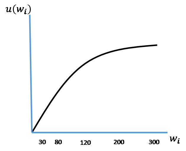
In Figure 3.1 below, we depict $u\left(w_i\right)=\sqrt{w_i}$ defined on a continuum from the lowest total wealth of $0 at the graph’s origin to the largest total wealth of $300. We also indicate the other total wealth levels of $30, $80, $120, and $200 associated with lotteries $L^\prime$ and $L^{\prime\prime}$ . Note that $\ u\left(w_i\right)=\sqrt{w_i}$ indeed exhibits diminishing marginal utility in $w_i$ , or to state it yet another way, $\ u\left(w_i\right)=\sqrt{w_i}$ is “concave” in $w_i$ .

Figure 3.1. Utility Function Defined Over Wealth Levels

For sake of example, let’s now superimpose the values associated with lottery $L^\prime$ on this graph, as shown in Figure 3.2.

Figure 3.2. Utility Function Defined Over Wealth Levels with Superimposed Lottery Values.

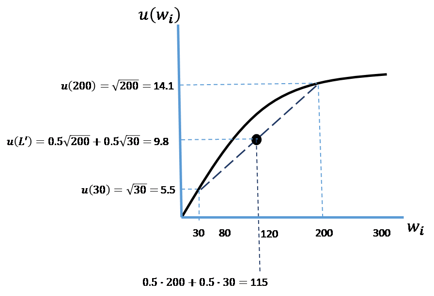
Begin by noting that with lottery $L^\prime$ the individual’s total wealth when she wins equals $200 (which, as indicated on the graph’s vertical axis, corresponds to $u\left(200\right)=\sqrt{200}$ = 14.1 utils), and equals $30 when she loses (corresponding to $u\left(30\right)=\sqrt{30}$ = 5.5 utils). We already know from the information provided in the example that $U\left(L^\prime\right)=0.5\sqrt{200}+0.5\sqrt{30}$ = 9.8 utils, as indicated on the graph’s vertical axis. What the example did not tell us is that the midpoint on the line segment connecting the individual’s utility values at lottery $L^\prime$ ’s loss outcome of $30 and win outcome of $200 corresponds to (0.5 x $200) + (0.5 x $30) = $115.^[1]

We can identify two values in this graph that provide quantitative measures of an individual’s risk aversion. As shown in Figure 3.3, the measures are known as “certainty equivalent” and “willingness-to-pay” (WTP) to avoid having to play the lottery in the first place.

Figure 3.3. Certainty Equivalent and WTP

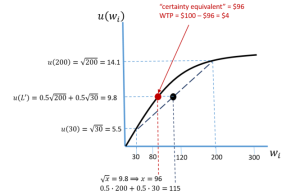
As depicted in the graph, the individual’s certainty equivalence is found by drawing a line horizontally from the midpoint of the line segment to its intersection with the utility function. Mathematically, this intersection corresponds to the value of $w_i$ (in the graph denoted as $x$ ) that solves for the expected utility value of lottery $L^\prime$ , 9.8 utils. This value is $96, which, because the individual in this example is risk averse, is less than $115.^[2] The individual’s WTP is then calculated as $100 – $96 = $4. In other words, the individual is willing to pay $4 (out of his initial wealth of $100) to avoid having to play lottery $L^\prime$ in the first place.

Before leaving this discussion of the expected utility form, consider the following thought experiment:

Choose between lotteries A and B:

A 80% chance to win $4,000
B win $3,000 for certain

If you chose lottery B, then you are considered risk averse. That’s because the expected value of playing lottery A (0.8 x $4,000 = $3,200) is larger than the certain value of lottery B, $3,000. If you weren’t averse to risk you would have chosen lottery A.

Because we are precluded from ever deriving your utility function, we cannot calculate your certainty equivalence, per se. So, this type of thought experiment proffers an admittedly expedient way to gauge whether you are risk averse. Can you think of an alternative experiment that would enable us to actually obtain your certainty equivalence?^[3]

Homo Economicus and the Indifference Curve**

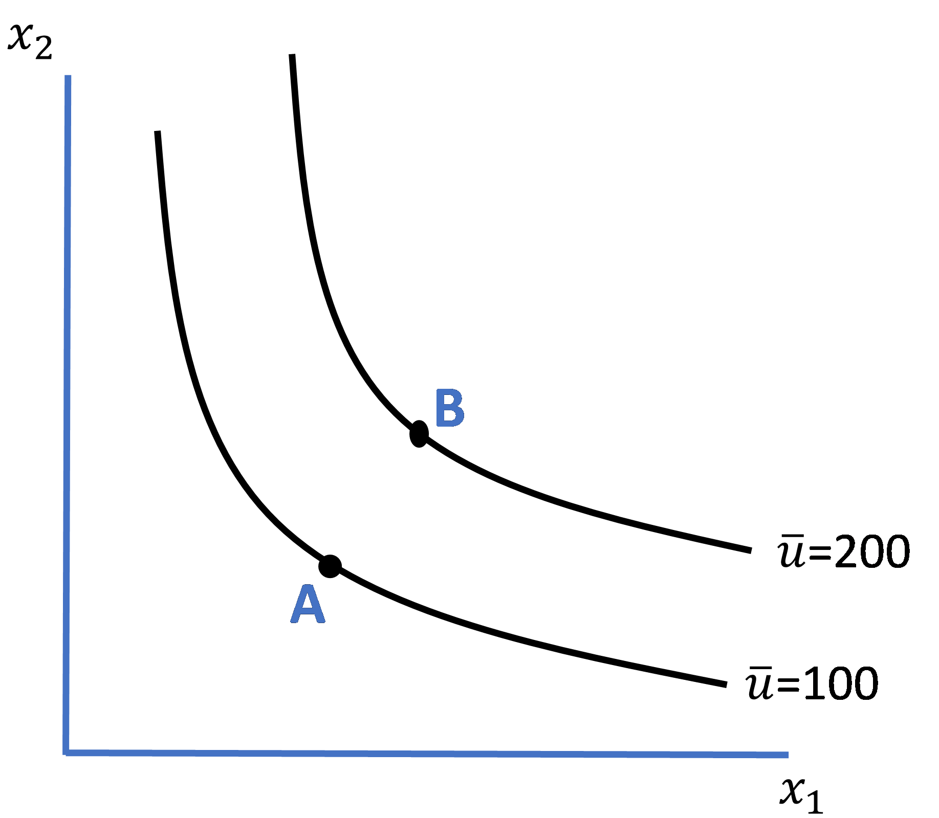
Before concluding this chapter on the rationality of Homo economicus, we introduce another important concept in Figure 3.4—the “indifference curve.” In doing so, we depart from the world of expected utility defined over Homo economicus’ possible wealth levels and venture into a world where Homo economicus chooses different levels of actual commodities to consume. In other words, we model Homo economicus’ choices in the context of a marketplace rather than the context of a lottery.

Figure 3.4. Homo economicus’ Indifference Curves

In Figure 3.4, let variables $x_1$ and $x_2$ represent the physical amounts of any two commodities 1 and 2 that Homo economicus might choose to consume (as a bundle) at some given point in time, and constant $\bar{u}$ represent some predetermined utility level, say 100 utils. An indifference curve defined for $\bar{u}$ = 100 depicts the tradeoffs Homo economicus is willing to make between the respective amounts of commodities 1 and 2 that still result in 100 utils of utility.^[4] Or, alternatively stated, the indifference curve depicts all of the bundles that yield Homo economicus the same utility level $\bar{u}$ = 100. Thus, Homo economicus would feel indifferent about owning any of the bundles on the indifference curve. Hence its name.

For those of you with a background in microeconomic theory, you will recall the stylistic version of Homo economicus’ indifference curves as shown in Figure 3.4. By “stylistic” we mean that the curves are everywhere downward-sloping and convex (i.e., bowed-out) from the graph’s origin. In this graph, we have drawn two indifference curves for the same individual—one corresponding to a utility level of 100 utils, the other to a utility level of 200 utils. It is no coincidence that the indifference curve associated with $\bar{u}$ = 200 lies everywhere above (to the northeast of) the indifference curve associated with $\bar{u}$ = 100. It is also no coincidence that the two curves are “well-behaved” (i.e., they are parallel and do not intersect each other).^[5]

The reason why the indifference curve lying to the northeast is associated with larger utility is because of what is known as monotonicity, specifically the assumption cum property that an individual obtains more utility by consuming larger amounts of the commodities. Recalling that a given indifference curve depicts all of the different bundles of goods (in our case bundles of goods 1 and 2) that provide an individual with the same level of utility, if we pick any bundle on curve $\bar{u}$ = 100 (say, bundle A), we can always find a bundle on curve $\bar{u}$ = 200 (say, bundle B) that includes more of both goods and thus, by the Monotonicity Property, implies that utility is indeed higher on $\bar{u}$ = 200.

The fact that Homo economicus’ indifference curves for $\bar{u}$ = 100 and $\bar{u}$ = 200 in Figure 3.4 do not intersect bears further mention. To see why, we need to recast our previous definition of the Transitivity Axiom we learned about in the context of lotteries to the context of commodities 1 and 2. As a reference point for the Transitivity Axiom, recall the earlier definition provided in the context of lotteries: if $L\succsim L^\prime$ and $L^\prime \succsim L^{\prime\prime}$ , then $L\succsim L^{\prime\prime}$ . In other words, if an individual weakly prefers lottery $L$ to lottery $L^\prime$ , and also weakly prefers lottery $L^\prime$ to lottery $L^{\prime\prime}$ , then it must also be the case that the individual weakly prefers lottery $L^\prime$ to lottery $L^{\prime\prime}$ . In the case of actual commodities, this definition of the Transitivity Axiom changes as follows: if an individual weakly prefers commodity bundle A to bundle B, and also weakly prefers bundle B to bundle C, then it must be the case that the individual weakly prefers bundle A to bundle C as well. See the parallel between these two contexts?

Now, assuming both the Transitivity Axiom and Monotonicity Property hold—as they do for Homo economicus—we can prove by contradiction that $\bar{u}$ = 100 and $\bar{u}$ = 200 do not intersect. Or, to state it another way, we can show that if the two curves do intersect, then transitivity and monotonicity cannot hold simultaneously. To see this, consider Figure 3.5 below, which includes two purposefully unlabeled indifference curves and three different consumption bundles A, B, and C.

Figure 3.5. A Violation of the Transitivity Axiom

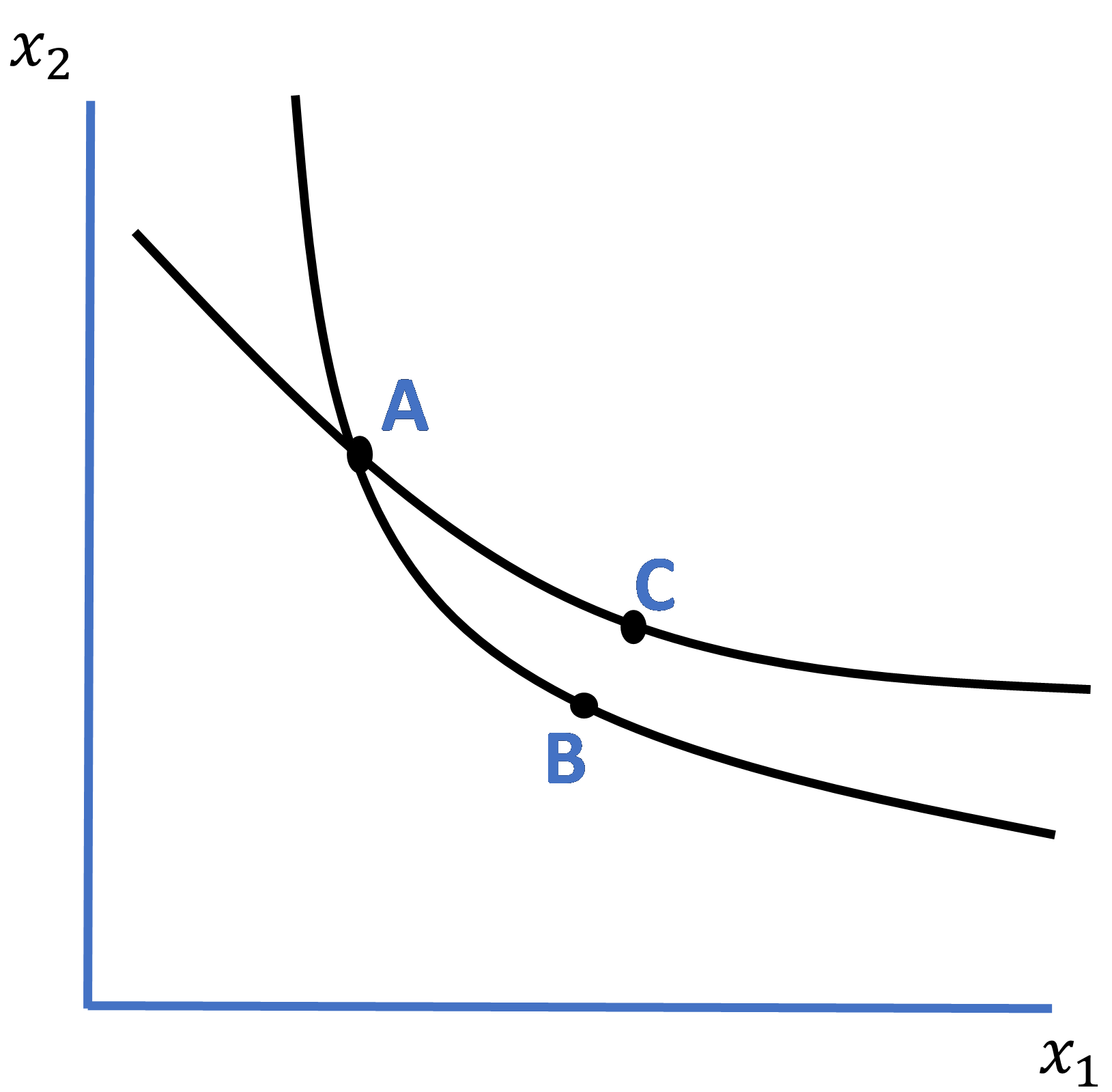
Begin by noting that, via the definition of an indifference curve itself, because bundles A and B lie on the same indifference curve, the individual prefers the two bundles equally (i.e., obtains the same level of utility from each bundle). Similarly, because bundles A and C lie on the same indifference curve, the individual also values these two bundles equally. Now, according to the Transitivity Axiom, it must be the case that the individual prefers bundles B and C equally as well. But wait, by the Monotonicity Property, bundle C lies to the northeast of bundle B and therefore has more of both goods 1 and 2 in its bundle. So, this property tells us that the individual instead prefers bundle C over bundle B, which contradicts the earlier conclusion reached by the Transitivity Axiom. Hmmm. We have a contradiction here, one which cannot stand. Thus, the indifference curves cannot intersect each other when the Transitivity Axiom and Monotonicity Property hold simultaneously. Alternatively stated, the indifference curves for Homo economicus cannot intersect.

Homo economicus and Intertemporal Choice***

The previous analyses of Homo economicus’ preferences and choice behavior have been strictly “static” in the sense that we have restricted our representative individual to making decisions during a single time period: the here-and-now. But decisions are typically not made in such a vacuum time-wise. Instead, we (both Homo economicus and Homo sapiens) consider how decisions made today will affect future decisions. In other words, we take into account how money spent today (e.g., for a new shirt) will affect our ability to purchase something else in the future (e.g., the latest book about behavioral economics). Choices that span multiple time periods—not just the here-and-now, but also the ‘there-and-later’—are known as “intertemporal,” and the analysis of these choices is “dynamic” rather than static.

Certainly, the span of time we could conceivably account for in our dynamic analysis of Homo economicus’ intertemporal choices is long, an entire lifetime. But to keep things tractable, and yet enable key comparisons between the intertemporal choice behavior of Homo economicus and (later, in Chapter 6) Homo sapiens, we make some simplifying assumptions. First, the time span under consideration is three periods rather than what could instead be considered a lifetime, or effectively an infinite number of periods.^[6] Second, we assume preferences are stable, in particular, that the individual’s utility function does not change shape (i.e., functional form) from one period to the next. Lastly, we assume that the individual’s annual income level remains constant over time, as do relative prices. As a result, our analysis loses no generality by assuming that all prices are normalized to a value of one.

These last two assumptions imply that Homo economicus exhibits perfect foresight, which should come as no surprise. Perfect foresight means that Homo economicus can accurately predict how her preferences, annual income, or prices of the different commodities will change over time, and thus account for these changes in her decision problem at the outset. Therefore, Homo economicus cannot be ‘tricked’ into making what appear to be inconsistent choices over time.

To see this, recall our earlier definition of an individual’s utility function, which allows us to model Homo economicus’ three-period intertemporal decision problem as follows,

$\begin{matrix}Max\\\left\{x_1,x_2,x_3\right\}\\\end{matrix}\ \ u\left(x_1\right)+\delta u\left(x_2\right)+\delta^2u\left(x_3\right)$

Subject to,

$W=\left(p_1\cdot x_1\right)+\left(p_2\cdot x_2\right)+\left(p_3\cdot x_3\right)$

where $x_1,x_2$ , and $x_3$ represent the amount of a composite consumption good consumed by the individual in each period 1, 2, and 3, respectively; function $u\left(\cdot\right)$ represents the individual’s utility defined over a given period’s consumption level; parameter $0<\delta\le1$ represents the individual’s “discount factor,” indicating the extent to which he is impatient for present, as opposed to future, consumption; prices $p_1,p_2$ , and $p_3$ are the given, constant prices for periods 1, 2, and 3, respectively; and aggregate income $W=3w,$ where $w=w_1=w_2=w_3$ (the string of equalities imposes the previously mentioned constant period-by-period income level).

As with the utility function defined earlier over an individual’s consumption bundle, the function $u\left(\cdot\right)$ is assumed to be increasing and concave in its respective period-by-period consumption levels. An impatient Homo economicus is represented by $\delta<1$ (yes, as with risk aversion, rational intertemporal choice theory permits Homo economicus to be an impatient consumer). As such, in solving her intertemporal decision problem (i.e., choosing at the outset $x_1,x_2$ , and $x_3$ to maximize aggregate utility across the three periods $u\left(x_1\right)+\delta u\left(x_2\right)+\delta^2u\left(x_3\right)$ ), Homo economicus discounts her second-period utility level more than her first-period’s, and in turn discounts her third-period utility more than her second period’s. Such is the nature of impatience in the context of an intertemporal choice problem.

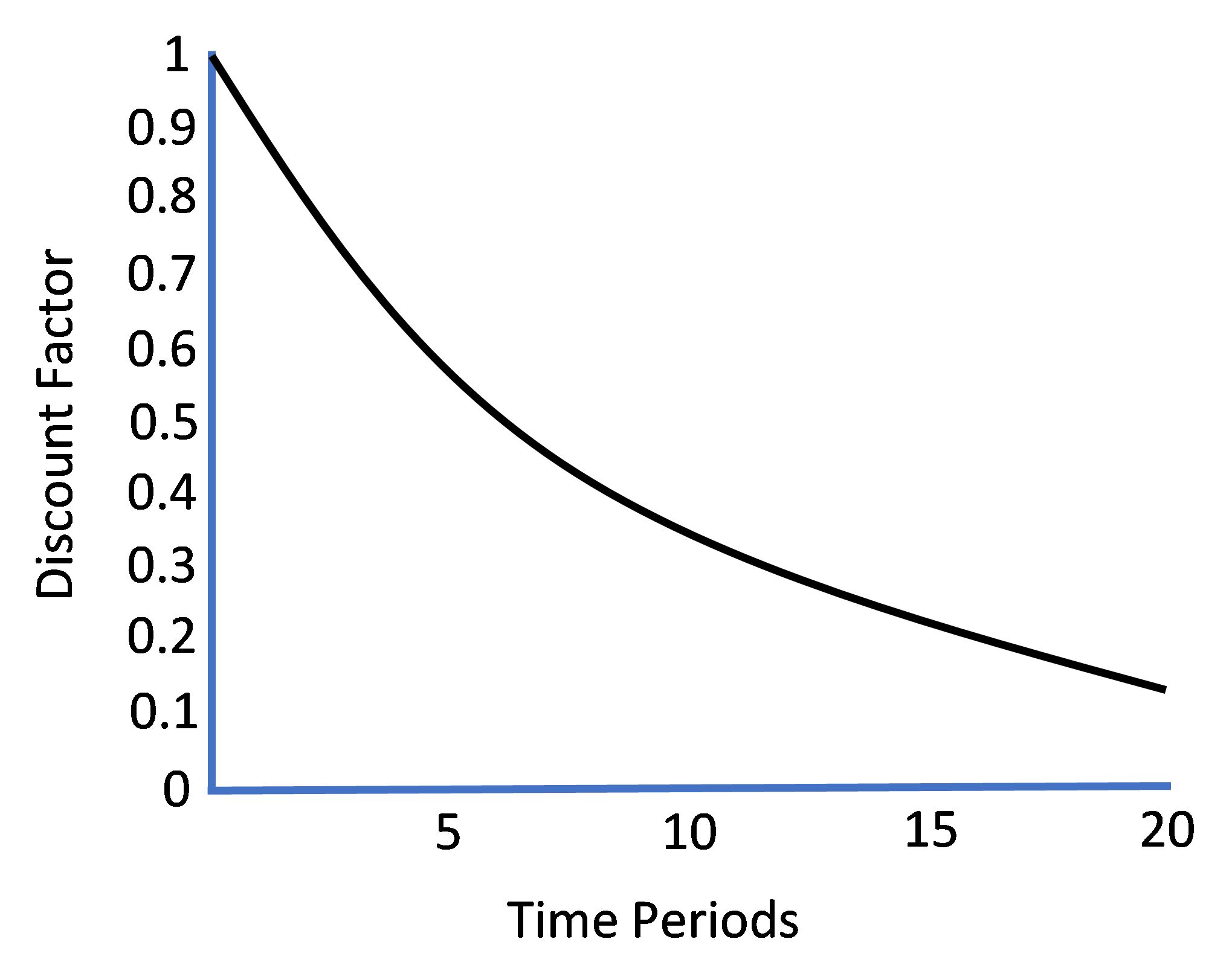
Because discount factor $\delta$ is constant across time but is nevertheless reduced in value through time exponentially (e.g., if there were a fourth period in our model, discounted utility would enter the individual’s aggregate utility as “ ${+\delta}^3u\left(x_4\right)$ ” and so on for additional periods), this pattern of discounting future utility is known as “exponential time discounting.” As Figure 3.6 shows below (for $\delta<1$ ), the schedule of ‘discounted’ discount factors over time charts out a negative exponential curve that is convex to the graph’s origin and asymptotically zero with respect to the passage of time. In other words, as time stretches out further into the future, future utility is discounted progressively to a point where Homo economicus severely minimizes the influence of additions to his aggregate utility obtained in the distant future.

Figure 3.6. Exponential Time Discounting

Three particular features of Homo economicus’ exponential discounting problem bear mentioning. First, in solving her intertemporal choice problem stated above, Homo economicus will optimally choose $x_1,x_2$ , and $x_3$ such that her discounted marginal utility levels are equated across time. Let these optimal levels of consumption be denoted $x_1^\ast,\ x_2^\ast$ , and $x_3^\ast$ , respectively. This result ensures a choice profile where $x_1^\ast>x_2^\ast>x_3^\ast$ , which is what we would expect the consumption profile of an impatient consumer to look like.

For those of you familiar with calculus, in particular solving constrained optimization problems, you will note that you can write this problem in its Lagrangian form as

$\mathcal{L}=u\left(x_1\right)+\delta u\left(x_2\right)+\delta^2u\left(x_3\right)+\lambda \left[W-x_1-x_2-x_3\right]$ ,

where $\lambda>0$ represents the problem’s Lagrangian multiplier, and for simplicity, we have normalized all prices to one (i.e., $p_1=p_2=p_3=1$ ). Obtaining the associated system of first-order conditions for this problem results in

$u^\prime\left(x_1\right)=\delta u^\prime\left(x_2\right)=\delta^2u^\prime\left(x_3\right)=\lambda$ ,

where $u^\prime\left(\cdot\right)$ denotes the individual’s marginal utility function. This string of equalities indicates that discounted marginal utility levels are equated across time. Given our underlying assumptions of $\delta<1$ and diminishing marginal utility, the string of equalities in turn implies $x_1^\ast>x_2^\ast>x_3^\ast$ .^[7]

Second, Homo economicus’ choice profile abides by what’s known as “stationarity.” In other words, her preferences for any increments to a given level of consumption in two different time periods depends upon the interval of time that passes between the two time periods (e.g., between periods 1 and 2), and not the specific points in time when the two respective increments could conceivably be consumed (e.g., periods 2 and 3).

For example, suppose Homo economicus chooses to consume the same base amount $x$ in each period, and let the two different increments to base consumption be denoted as $i_1$ and $i_2$ . Stationarity implies that if $u\left(x+i_1\right)>\delta u\left(x+i_2\right)$ , where $u\left(x+i_1\right)$ represents the corresponding utility level in period 1 and $\delta u\left(x+i_2\right)$ represents discounted utility level in period 2, then $\delta u\left(x+i_1\right)>\delta^2u\left(x+i_2\right)$ by exactly the same amount as $u\left(x+i_1\right)>\delta u\left(x+i_2\right)$ , where $\delta u\left(x+i_1\right)$ represents a discounted utility level in period 2 and $\delta^2u\left(x+i_2\right)$ represents a discounted utility level in period 3. This result is easy to see since $\delta u\left(x+i_1\right)>\delta^2u\left(x+i_2\right)$ for periods 2 and 3 reduces to $u\left(x+i_1\right)>\delta u\left(x+i_2\right)$ for periods 1 and 2 after cancelling $\delta$ from each side of the former inequality. Since the two inequalities are identical through time, Homo economicus’ preferences are stationary through time.

Note that the time intervals under comparison must be of equal length for stationarity to be assessed. For example, if $u\left(x+i_1\right)>\delta u\left(x+i_2\right)$ for consecutive periods 1 and 2, this does not necessarily imply that $u\left(x+i_1\right)>\delta^2u\left(x+i_2\right)$ by the same amount across non-consecutive periods 1 and 3 (convince yourself of this fact). To further test your understanding of stationarity, suppose there was a fourth period of consumption. You should be comfortable seeing that if $u\left(x+i_1\right)>\delta^2u\left(x+i_2\right)$ between periods 1 and 3, then $\delta u\left(x+i_1\right)>\delta^3u\left(x+i_2\right)$ between periods 2 and 4 by the same amount.

Third, Homo economicus’ preferences are “time consistent,” In other words, given that he has chosen $x_1^\ast,\ x_2^\ast$ , and $x_3^\ast$ at the outset for any given set of $\delta$ , $W$ , and prices $p_1,p_2$ , and $p_3$ , then if after having consumed at level $x_1^\ast$ in period 1, the individual decides to re-solve his decision problem from that point forward (i.e., now starting in period 2), he will not deviate from choosing $x_2^\ast$ and $x_3^\ast$ . In this case, the individual effectively solves the two-period problem,

$\begin{matrix}Max\\\left\{x_2,x_3\right\}\\\end{matrix}\ \ u\left(x_2\right)+\delta u\left(x_3\right)$

subject to,

$W=2w=\left(p_2\cdot x_2\right)+\left(p_3\cdot x_3\right)$ ,

which results in the same $x_2^\ast$ and $x_3^\ast$ as before. To see this result, first note that we can pull $\delta u^\prime\left(x_2\right)=\delta^2u^\prime\left(x_3\right)$ from the string of three equalities derived from the individual’s original decision problem (i.e., $u^\prime\left(x_1\right)=\delta u^\prime\left(x_2\right)=\delta^2u^\prime\left(x_3\right)$ ) and then cancel $\delta$ from each side of the equality, resulting in $u^\prime\left(x_2\right)=\delta u^\prime\left(x_3\right)$ . But $u^\prime\left(x_2\right)=\delta u^\prime\left(x_3\right)$ is precisely the equality that results from the first-order conditions for this two-period problem. Given that nothing else has changed in this problem (i.e., the values for $\delta$ , $w$ , and $p_1,p_2$ , and $p_3$ are the same, as is the functional form of $u\left(\cdot\right)$ and the fact that $x_1^\ast$ has already been chosen), no values for $x_2$ and $x_3$ , respectively, solve $u^\prime\left(x_2\right)=\delta u^\prime\left(x_3\right)$ except $x_2^\ast$ and $x_3^\ast$ .

And if after having consumed at levels $x_1^\ast$ and $x_2^\ast$ for the first two periods, he then decides to re-solve his decision problem from that point forward (i.e., now starting in period 3), he does not have a problem left to solve—he has effectively locked himself into consuming $x_3^\ast$ at that point. Therefore, because he chooses not to alter his consumption profile over time by having embarked on these period-by-period decision problems, we say that his choices are time consistent.

Key Takeaways on Homo economicus

So, what have we learned about Homo economicus thus far? For starters, we have learned that she is inviolable when it comes to making the miscalculations and misjudgments, exhibiting the biases, and falling victim to the fallacies and effects that bedevil Homo sapiens. Furthermore, Homo economicus is inextricably bound by the rationality axioms of Completeness, Transitivity, Dominance, Invariance, Independence, Substitutability, and the Sure-Thing Principle. And when confronted with the uncertainty of having to play a lottery, Homo economicus chooses to maximize expected utility derived over her total wealth. In the face of uncertainty, Homo economicus can be risk averse. And when it comes to a deterministic setting, such as when Homo economicus enters the marketplace to purchase actual commodities, the family of indifference curves that represent her preferences for different bundles of commodities are not permitted to intersect with each other.

In other words, Homo economicus is—to borrow the title of Sade’s hit song—a smooth operator. Her expected utility function and indifference curves are smooth, and when it comes to navigating the challenging choice situations that often confound Homo sapiens, she smoothly averts the pitfalls. Nevertheless, as we pivot to learning about the behavioral economic theories that have emerged to explain the divergences in choice behavior between the two species, bear in mind that to a great extent the reason why Homo economicus seems so smooth is because the world explained by the rational choice model is perforce restrictive of many of the characteristics that define the human experience—emotion, sensation, distraction, a world whose complications seem to demand imperfection and roughness (as opposed to smoothness). As a result, Homo economicus couldn’t help but perform well within a bubble of surreality. Fortunately, as we are about to learn, the adjustments to the rational-choice framework devised by behavioral economists are quite efficacious, not to mention eloquent.

Study Questions

Note: Questions marked with a “‡” are adopted from Cartwright (2014).

State the Completeness and Independence Axioms in two separate, easy-to-understand sentences.
Recall that Figures 3.1 – 3.3 are depicted for utility function $u\left(w_i\right)=\sqrt{w_i}$ , indicating that Homo economicus exhibits “risk aversion” with respect to total wealth level . (a) Suppose instead that $u\left(w_i\right)=w_i$ . Reconstruct Figures 3.1 – 3.3 for this utility function and interpret your results in relation to the figures in the text derived for $u\left(w_i\right)=\sqrt{w_i}$ . Can you think of any reason why $u\left(w_i\right)=w_i$ might not be representative of Homo economicus’ preferences? Explain. (b) Now let $u\left(w_i\right)=w_i^2$ . Reconstruct Figures 3.1 – 3.3 for this utility function and interpret your results in relation to the figures in the text derived for $u\left(w_i\right)=\sqrt{w_i}$ as well as those you derived in part (a) for $u\left(w_i\right)=w_i$ . Can you think of any reason why $u\left(w_i\right)=w_i^2$ might not be representative of Homo economicus? Explain.
^‡ Suppose Henry the Homo economicus is presented with the following lotteries: Lottery A: Win $6,000 with a probability of 0.45. Lottery B: Win $3,000 with a probability of 0.9. Lottery C: Win $6,000 with a probability of 0.001. Lottery D: Win $3,000 with a probability of 0.002. Show why it would be inconsistent for Henry to choose Lottery B over Lottery A together with Lottery C over Lottery D. What pattern do you notice in the four lotteries?
In Figures 3.4 – 3.5, Homo economicus’ indifference curve is drawn downward-sloping. Suppose instead that the indifference curve is upward-sloping, as depicted in the figure below. Interpret this figure. Hint: One of the two goods is actually a “bad” rather than a “good.” Would Homo economicus ever exhibit an upward-sloping indifference curve?
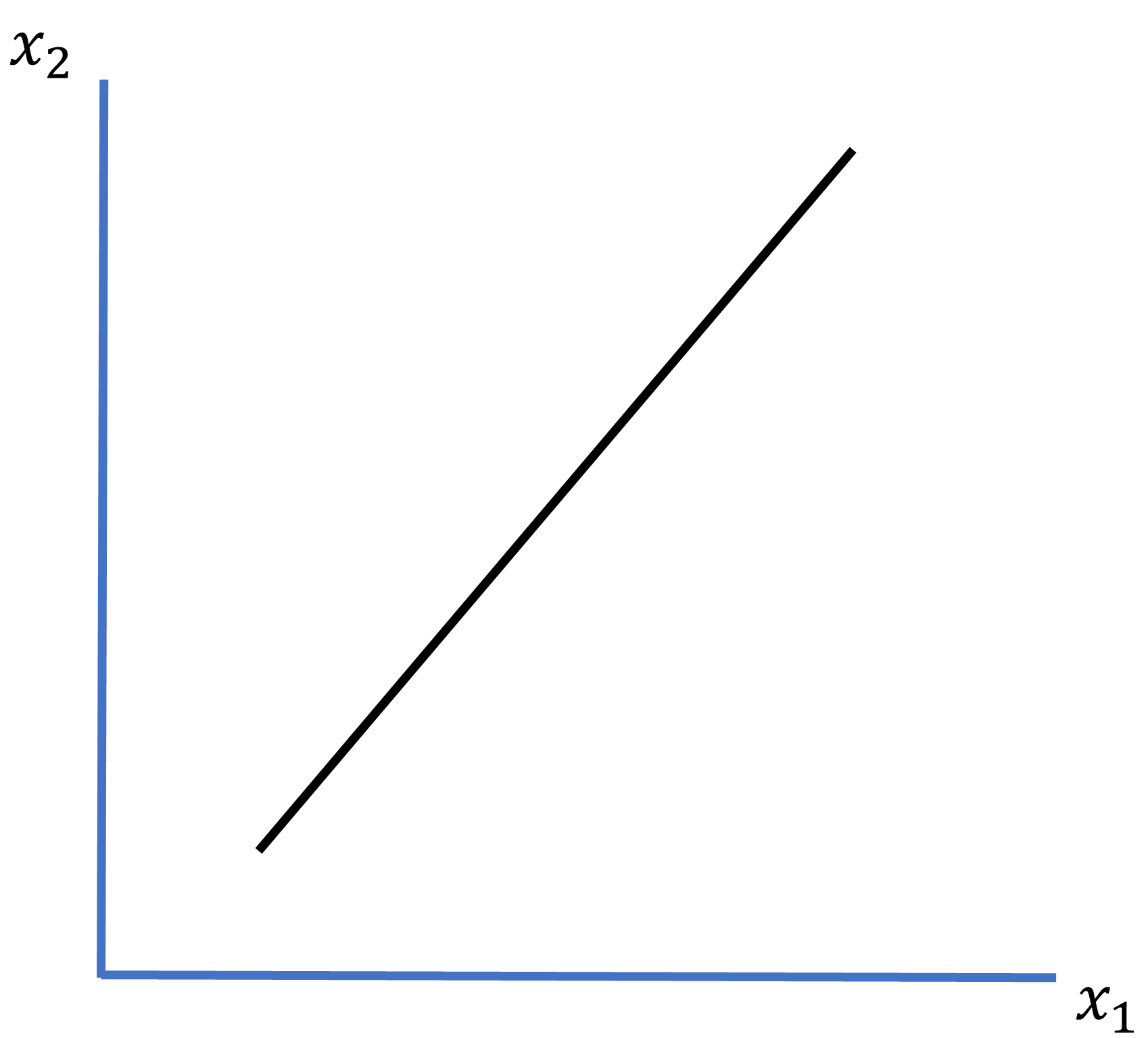
Given the upward-sloping indifference curve in Question 4, does satisfying the Transitivity Axiom still imply that indifference curves cannot intersect one another? Explain.
What does satisfying the Invariance Axiom imply about Homo economicus’ susceptibility to Framing Effects studied in Chapter 1?
What does satisfying the Sure-Thing Principle imply about Homo economicus’ susceptibility to Priming Effects studied in Chapter 1?
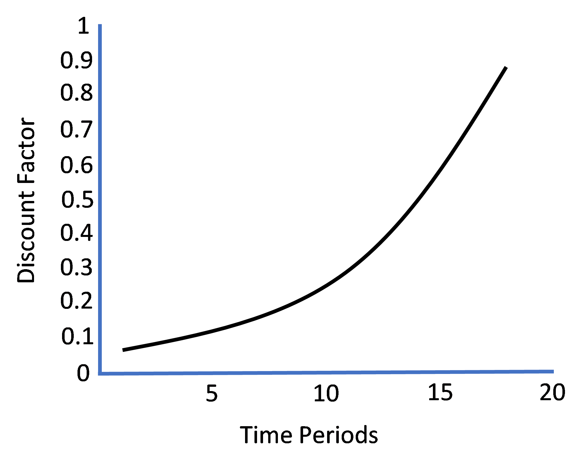
What would you call an individual whose time discounting path is depicted in the figure below (i.e., it fits the shape of a positive exponential curve rather than negative exponential curve as depicted in Figure 3.6)?

Media Attributions

Figure 3.3v3

Note that our reference point for this example—the midpoint of the line segment—corresponds to lottery $L^\prime$ ’s 50%-50% split in probability of a win and a loss. If, for example, the lottery’s split had instead been 60%-40% in favor of winning, then the reference point would be located further to the northeast on the line segment, corresponding to a $w_i$ of 0.6 x ($200 + $30) = $138. ↵
By contrast, if the individual had been assumed “risk neutral,” in which case her utility function would be drawn linear with respect to wealth $w_i$ , certainty equivalent would per force be equal to $115. What would be the result if our individual was instead “risk seeking,” also known as “risk loving”? ↵
Suppose I would have confronted you with the following lottery: 80% chance of winning $4,000 and 20% chance of losing $3,000. I then ask you two questions: (1) what is your initial wealth, and (2) what are you willing to pay to avoid having to play this lottery (WTP)? Suppose you answer that your initial wealth is $10,000 and your WTP is $100. Recalling our previous graphical analysis, we could stop right here. Because your WTP is greater than zero, we know that for this particular lottery, you are risk averse. But we can also go a bit further and calculate your corresponding certainty equivalence for this lottery. From our graphical analysis we learned that certainty equivalence is the difference between your expected total wealth from playing the lottery and your WTP. Given that your initial wealth is $10,000, and you have an 80% chance of winning $4,000 and a 20% chance of losing $3,000, your total expected wealth from playing the lottery is (0.8 x $14,000) + 0.2 x $7,000) = $12,600. Subtracting your WTP of $100 from $12,600 results in a certainty equivalence of $12,500. ↵
For those of you who have seen indifference curves before, recall that the slope of the indifference curve at any given bundle of commodities $x_1$ and $x_2$ is the curve’s marginal rate of substitution (MRS), which can be shown to equal the negative ratio of the individual’s marginal utilities at that bundle. The MRS, then, is a marginal or continuous measure of the rate at which the individual is willing to tradeoff commodity 2 for more of 1. ↵
The shape and location of the indifference curve is directly related to the individual’s utility function as it is defined over $x_1$ and $x_2$ . For example, it can be shown that indifference curves such as those depicted in the figure can be derived from what’s known as a Cobb-Douglas utility function, where $u\left(x_1,x_2\right)=\sqrt{x_1x_2}$ . ↵
Technically speaking, only two time periods are necessary to conduct dynamic analysis (e.g., today and tomorrow, or this year and next year). Hence, we could claim that our three-year time span extends beyond what is necessary here. ↵
Since $x_1^\ast>x_2^\ast>x_3^\ast$ in the face of the underlying assumption that $w_1=w_2=w_3$ , we effectively assume the individual borrows against future income (without interest penalty) to obtain the larger consumption level in period 1. Because the roles of borrowing and saving are extraneous to the insights we seek from the individual’s choice problem, we lose nothing by casting the borrowing and savings decisions as implicit. ↵

License

Icon for the Creative Commons Attribution 4.0 International License