7 Some Classic Games of Iterated Dominance
Before diving into the deep pool of behavioral game theory, we need some specific nomenclature about what constitutes a game and its solution, or what we have been calling its equilibrium. If you’ve ever played a board or card game with your friends or family, then none of this terminology should surprise you.
A game consists of a set of “players,” each with their own set of “strategies.” Precise “rules” govern the “order” in which players make their “moves,” the “information” they have available, and, ultimately, their “payoffs.” I don’t know about you, but the card game poker comes immediately to mind. The keywords are players, strategies, rules, order, moves, information, and payoffs.
We expect that Homo economicus will attain what’s known as a Nash equilibrium, or perhaps a refinement of Nash equilibrium, depending upon the game being played.[1] Simply put, a Nash equilibrium prevails when each player can no longer adjust his or her strategy to obtain added payoff. Thus, in a Nash equilibrium, all players have chosen respective strategies that are the best responses to each of the other players’ strategies. The Nash equilibrium is derived analytically and, thus, is highly predictable. We will see just how predictable the equilibrium is in a wide variety of games. Since this is the equilibrium obtained by Homo economicus, we henceforth use the terminology Homo economicus and “analytical equilibrium” inter-changeably.
As we will learn, the equilibria typically obtained in games played by Homo sapiens expand upon the Nash equilibrium concept by adding in such aspects of the human experience as emotion, miscalculation, limited foresight, doubt about how informed the other players are, and learning-by-doing—many of the same human quirks and idiosyncrasies we encountered in Section 1. The equilibria obtained in games played by Homo sapiens are typically derived more intuitively than analytically. Thus, the equilibria are generally unpredictable.
Let’s start with one of the most famous and basic of games—ultimatum bargaining.
Ultimatum Bargaining
Consider the following game presented in Camerer (2003):[2]
 , of the $100 to the Responder, leaving the Proposer with $(100 – ). If the Responder accepts the offer, then she gets $ and the Proposer gets $(100 – ). If the Responder rejects the offer, both players get nothing.
The analytical equilibrium for this game evolves according to the following logic:
By going first, the Proposer possesses all of the bargaining power. The Proposer, therefore, exploits the fact that the self-interested Responder will take whatever is offered. The amount offered by the Proposer is thus very close to zero. Surmising that this is indeed the Proposer’s best strategy, and also recognizing that he gets nothing if he rejects the Proposer’s offer, the Responder has no better strategy than to accept whatever the Responder offers, as meager as the offer is. The Proposer knows that this is the logic the Responder will use, and the Proposer knows that the Responder knows this, and so on. Hence, the analytical equilibrium is that the Proposer makes the meager offer (in the limit, $0.01) and the Responder accepts.
Ouch. Before exploring what the behavioral game theory literature has to say about how Homo sapiens have actually played this game (i.e., what equilibria they have obtained), it is informative to link this game to the nomenclature presented at the chapter’s outset.
The players are a Proposer and Responder. The Proposer’s strategy is to choose an offer amount, , that he thinks will ultimately be accepted and result in a desired payoff amount. The Responder’s strategy is to accept or reject the Proposer’s offer. The rules of the game, which govern which player moves when (i.e., the order of moves) and how the resulting payoffs are determined, are clearly spelled out. The Proposer moves first by making offer and the Responder moves second, choosing to accept or reject the offer. After the Responder’s decision is made, the payoffs are distributed according to the following rule: If the Responder accepts the Proposer’s offer, the payoffs are for the Responder and  for the Proposer; if the Responder rejects the Proposer’s offer then the payoffs are zero for each.
As the logic behind the determination of the analytical equilibrium makes clear, the information available to the Proposer and Responder has an important bearing on the game’s analytical equilibrium. Although this game has allocated all of the bargaining power to the Proposer, both the Proposer and the Responder are assumed to share complete and common information. Each player not only knows what payoffs he stands to gain via the game’s rule, but also what payoffs the other player stands to gain, and each player knows that the other player knows this, and so on. The fact that all players know the same things about the game is what is common about the information. The fact that no information is hidden from the players is what makes the information complete.
The solution process for the Ultimatum Bargaining game’s analytical equilibrium follows what’s known as “iterated dominance” due to (1) the players making their moves sequentially (or iteratively), and (2) the concomitant need for each player to think ahead about the other player’s subsequent move before choosing what to do presently. In this case, because each player’s best strategy is calculatable and unique, we say that it is dominant.[3] Further, because the Proposer in this game initially considers what should happen in the last stage, where the Responder decides whether to accept or reject the offer made in the first stage, iterated dominance is operationalized via “backward induction.” The Proposer first figures out what should be the outcome of the game’s final stage and then works back from there to determine what she should do in each preceding stage all the way back to the first stage. Because the equilibrium is solvable via backward induction, we say that it is “subgame perfect.”[4] We will be seeing examples of backward induction and subgame perfection repeatedly in this chapter, so get ready!
From an analytical, game-theoretic perspective, this is all interesting to know. But what about Homo sapiens? How have we actually played the Ultimatum Bargaining game? We have several different kinds of results. Camerer (2003) has compiled an exhaustive list of studies that have considered ultimatum bargaining with varying rules, payoff amounts, and multiple rounds, in different regions of the world with varied cultural contexts, with men vs. women, and more. He concludes that results from the different versions of the game are quite robust. Modal and median ultimatum offers are usually 40%–50% of the total amount available to bargain over, and means are 30%–40%. There are hardly any offers made by the Proposer in the outlying category of 0%-10%, and the hyper-fair category 51%–100%. Offers of 40%–50% are rarely rejected. Offers below 20% or so are rejected about half the time (Camerer, 2003).
In other words, Homo sapiens do not generally converge to the game’s analytical equilibrium. It seems that Proposers are susceptible to emotions like guilt, fairness, and/or altruism, and Responders succumb to envy and fairness (in this case, “reciprocity”). Here is a taste of some of the findings:
- Ironically, participants in more-primitive cultures in Africa, the Amazon, Papua New Guinea, Indonesia, and Mongolia have been found to behave more like Homo economicus than do participants in less-primitive cultures in the US, Europe, and Asia (c.f., Slonim and Roth, 1998; Buchan et al., 2004; Henrich et al., 2001 and 2002; Henrich, 2000).
- Repeated games with “stranger matching” and no provision of “history of moves” show a slight tendency for both offers and rejections to fall over time. Provision of history correlates with more pronounced reductions in offers and rejections (c.f., Roth et al., 1991; Bolton and Zwick, 1995; Knez and Camerer, 1995; Slonim and Roth, 1998; List and Cherry, 2000).
- Responders are not necessarily more likely to reject, say, $5 out of $50 than $5 out of $10, and similarly 10% of $50 than 10% of $10. In other words, the game’s stakes do not necessarily matter (c.f., Camerer and Hogarth, 1999; Roth et al., 1991; Forsythe et al., 1994; Hoffman et al., 1996; Straub and Murnighan, 1995; Cameron, 1999; Slonim and Roth, 1998).
- Male Proposers do not necessarily offer more to attractive female Responders, but female Proposers have been found to offer more to attractive male Responders (Hamermesh and Biddle, 1994).
- Young children are more self-interested, Homo economicus-like Proposers and Responders, but then become more fair-minded as they grow older (Damon, 1980; Murnighan and Saxon, 1998; Harbaugh et al., 2000).
- Calling the game a “seller-buyer exchange” encourages self-interest. Describing the game as a “common pool resource” encourages generosity (Hoffman et al., 1994; Larrick and Blount, 1997). Note that this is an example of a framing effect!
- When Proposers know the exact amount of money to be divided, and Responders either know nothing at all or know the probability distribution of possible amounts, Proposers offer less (c.f., Huck, 1999; Camerer and Loewenstein, 1993; Mitzkewitz and Nagel, 1993; Straub and Murnighan, 1995; Croson, 1996; Rapoport et al., 1996). This is a consequence of “incomplete information.” However, when Responders know the alternative amounts that the Proposer could have offered, they tend to exhibit “inequality aversion” (or, alternatively, a commitment to fairness) and reject the Proposer’s offer (Falk et al., 2003).
- Creating a sense of entitlement by letting the winner of a contest (played beforehand) be the Proposer lowers offers (c.f., Hoffman et al., 1994; List and Cherry, 2000). This is known as an Entitlement Effect.
Raworth (2017) eloquently sums up the main takeaway from these disparate findings: Homo sapiens’ sense of reciprocity appears to co-evolve with their economy’s structure, or if you like, the context within which the game is played. In addition to the varied contexts described above, the structure of the Ultimatum Bargaining game has been modified as well. We consider two of these structurally adjusted versions of the game—the Nash Demand Game and the Finite Alternating-Offer Game.
Nash Demand Game
Consider the following game proposed by Mehta, et al. (1992):
The analytical equilibrium for this game obtains evolves according to the following logic:
Since Homo economicus know the composition of the deck, one player can tell from his own hand how many aces the other player has—namely, four minus his own number of aces. Thus, in the second stage, the players should always trade with each other such that the four aces end up being held by one of the players, as this gives them the right to state their demands in the third and final stage. Recognizing that the cards were randomly dealt to begin with, the players should each state a demand of $5 in the final stage.
What happens when Homo sapiens play the Nash Demand (ND) game instead? Mehta, et al. provide an answer. The authors start by considering what happened when Player 1 was dealt two aces in the first stage of their experiment. Of the 42 instances where this happened, 40 resulted in the player ultimately demanding half the pie of $10 in the final stage of the game. Thus, Player 1 behaved as would be expected of Homo economicus. However, when Player 1 was dealt either one ace or three aces, she demanded half the pie only roughly half of the time—16 of 32 times when dealt one ace and 17 of 33 times when dealt three. The other half of the time, Player 1 demanded a fraction roughly equal to the fraction of aces originally held—16 of 32 times when dealt one ace and 15 of 33 times when dealt three. As a result, there is a 22% ((16/32) x (15/33) = 0.22) deviation from the analytical equilibrium (of an even split in demands) in cases where one and three aces have been dealt to Player 1.
Mehta, et al. postulate that the implicit information about how many aces each player originally held in the ND Game created “focal points” for this type of deviation. For example, when Player 1 was dealt one ace and three deuces she was able to discern that Player 2 held the other three aces and one deuce. In those instances, Player 1 determined that because she contributed only one of four aces now held by Player 2 she should demand less than half of the $10. Similarly, when Player 1 was dealt three aces she should demand more than half of the $10.
In a slight twist on the basic ND game, Binmore et al. (1998) had their subjects play the game with an “outside option.” This game is played according to the same rules as the basic ND game except that before the game begins, Player 2 is randomly given a commonly known outside option worth $0.90, $2.50, $4.90, $6.40, or $8.10. In other words, before the game begins, Player 2’s outside option (which is equal to one of the five possible values stated in the previous sentence) is announced to both players. Player 2 can choose to take the option, in which case he gets that payment, and Player 1 gets nothing. Or Player 2 can turn down the option, and the ND game ensues.
A Homo economicus version of Player 1 should ignore Player 2’s outside option since if Player 2 turns down the option and opts to play the ND Game, then playing the game from that point forward is all that matters. Being a member of Homo economicus, Player 2 knows that this is indeed Player 1’s best strategy, and thus, if the ND game is ultimately played, Player 1 will demand $5, which means that the most Player 2 will be able to demand is also $5—the analytical equilibrium is therefore obtained. Hence, Player 2 will take the outside option only if it is worth $6.40 or $8.10. Otherwise, Player 2 should turn down the option and play the ND game with Player 1.
Binmore et al. found that Player 2s do not behave like Homo economicus. For instance, one-third of Player 2s opt out at the option value $4.90 and only 60% opt out at $6.40. Further, the demands of those Player 2s who opt-in at option values above $5.00 match those (focal) values rather than the expected $5.00. Player 1 behaviors deviate less from what we would expect of Homo economicus. Their demands are relatively close to $5.00 except in cases where Player 2’s option values exceed $5.00. Interestingly, Player 1’s demands decrease in accordance with the commonly known option values for Player 2, resulting in a total demand less than the $10 threshold. To the extent that Player 1 expects Player 2 demands to tilt toward the focal points of their option values, Player 1 is actually making a rational choice in lowering her demands. And to the extent that Player 2 with higher option values expects Player 1 to lower her demand accordingly, then Player 2 is likewise making a rational choice. The fact that relatively few Player 1s make demands that leave Player 2s with less than their option values is also rational to the extent that Player 1s expect Player 2 demands to tilt to their option values.
So, while the behavior of the players in Binmore et al.’s (1998) ND game with an outside option does not adhere to those expected in an analytical equilibrium, to the extent that their behaviors are premised on Homo sapiens’ tendencies to tilt toward focal points in these types of games we can interpret the players as nevertheless making contextually rational choices.
Finite Alternating-Offer Game
Consider the following game presented in Camerer (2003):
Solving this game analytically requires the use of backward induction, which results in a subgame perfect equilibrium (SPE). The logic goes like this:
Using backward induction, Player 1 considers what Player 2 will do in the second period when it is Player 2’s turn to make the counteroffer. Player 1 does not want the initial offer to be rejected since this will shrink the pie to $50. So, Player 1 offers at most $50 to Player 2 ($50 being the most Player 2 could ever hope to get if he rejects Player 1’s offer). Player 1, therefore, keeps at least $150 and Player 2 gets at most $50.
Camerer reports that in games played with Homo sapiens, Player 1 tends to offer half of the pie in the first stage (e.g., out of a sense of fairness or fear that the initial offer might otherwise be rejected by Player 2), in which case Player 2’s ability to reject the initial offer is perceived as a credible threat by Player 1. However, with repeated play, Player 1 quickly learns to offer the SPE amount of $50 in the first stage. In other words, as Homo sapiens learn how to play the game, Player 2’s threat is no longer perceived as being all that credible. Incredible, huh? With learning, Homo sapiens attain the analytical equilibrium.
Continental Divide Game
Consider the following game proposed by Van Huyck et al. (1997):
Players (more than two) each pick a number from 1 to 14. The rows of the matrix below show each player’s payoff (in dollars) corresponding to the number she has chosen and the median choice made by the group as a whole.
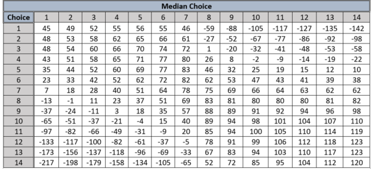
For example, if a player chooses 4 and the median is 5, the player earns a healthy payoff of $71. If the median is instead 12, the player earns -$14 (i.e., she loses $14)
Before discussing the logic behind the game’s analytical equilibrium, it is useful to point out where backward induction and subgame perfection factor into determining the equilibrium, if at all. It turns out that backward induction is actually a moot point in this game. This is because there is only a single stage—all players simultaneously choose their numbers, which then automatically determines the median number and attendant payouts. One might be tempted to say that there are  subgames, where
  represents the number of different players. This is not correct. There are instead possible outcomes to what is only a single subgame (the game itself).
The logic behind the game’s analytical equilibrium goes like this:
First, note that for any median less than or equal to 7, a player’s best response is to choose the number 3. This is because, being a member of Homo economicus, each player knows that every other player is both self-interested and thinking the same way. Thus, if each player chooses 7—which results in a median of 7—it will be in a given player’s self-interest to deviate and choose the number 5. But every player is equally self-interested and thinks the same way. Thus, a median of 5 results. But at a median of 5, each player deviates to the number 4. And at a median of 4, each player deviates to 3. Only at the choice of 3 does this madness stop. We call this the “low” Nash equilibrium. Using the same logic, for any median greater than 7 a player’s best response is to choose the number 12. We call this the “high” Nash equilibrium. We expect this game’s analytical equilibrium to be the high Nash equilibrium.
Van Huyck et al. played this game with 10 different groups of Homo sapiens, each group playing the game 10 times in a row. What they found were basins of attraction. For groups that start with a median of 7 in the first period, the equilibrium converges to medians of 3, 4, and 6 (i.e., there is an attraction toward the low Nash equilibrium). For groups that begin with a median greater than 7 in the first period, the basin of attraction leads toward medians of 12 and 13 (i.e., the high Nash equilibrium). Hence, while not all groups of Homo sapiens obtain the high Nash equilibrium, it seems that roughly half do. The outcome is what we call “path dependent”—dependent upon where the path begins.[5]
Beauty Contest
Consider the following game presented in Camerer (2003):
 players simultaneously chooses a number
  in the interval [0, 100]. The average for the group is calculated and then multiplied by a factor
  <1 (say, = 0.7). The player whose number is closest to this target (in this case, 70% of the average) wins $20.
Probably like you, the relationship between this game and a beauty contest escapes me.[6] But the game, regardless of what we call it, provides a nice example of how iterated dominance can be used to identify an analytical equilibrium.[7] The logic for the analytical equilibrium is as follows:
Each player starts by thinking, “Suppose the average is 50.” Given this, he chooses the number 35 (0.7 x 50). But he would not stop here (i.e., he would begin iterating). He realizes that everyone else is making the same calculation, so he will choose 25 instead (0.7 x 35). But wait. He would then choose 18 (0.7 x 25). But wait……he would ultimately choose zero, which is this game’s analytical equilibrium.
Camerer reports results for one Beauty Contest played by groups of Homo sapiens, where = 0.7 and there are low stakes of $7 and high stakes of $28. Irrespective of the stakes, Homo sapiens do not generally converge to the analytical equilibrium where each player chooses zero. But Homo sapiens do get close, especially when the stakes are higher. Camerer (2003) also reports that in most studies, players have used anywhere from zero to three levels of iterated dominance, which, according to the logic for the analytical equilibrium, means that the numbers most frequently chosen are 50, 35, and 25—quite a ways from zero.
Traveler’s Dilemma
Consider the following game proposed by Capra et al. (1999):
Applying iterated dominance, the logic for the analytical equilibrium goes like this:
Players should state claims that are one cent below what the other player is expected to state. In this way, a player helps boost the minimum claim (and hence her payoff) while earning the $50 reward. The result is a race to the bottom in which both players end up choosing the minimum claim of $300, and thus, neither player wins the reward (or, thankfully, suffers the penalty). This is the game’s unique Nash equilibrium.
Homo sapiens? Capra et al. found convergence toward the analytical equilibrium with their subjects over 10 periods of play only for the higher reward/penalty levels. In the later periods, average equilibrium claims were inversely related to the reward/penalty levels (the lower the reward/penalty level, the higher the average claim). Once again there is some evidence to suggest that Homo sapiens learn to converge toward (not necessarily all the way to) the analytical equilibrium, and the stakes of the game matter to some degree.
Escalation Game
Spaniel (2011) explores the Escalation Game, depicted below as a decision tree.[8]
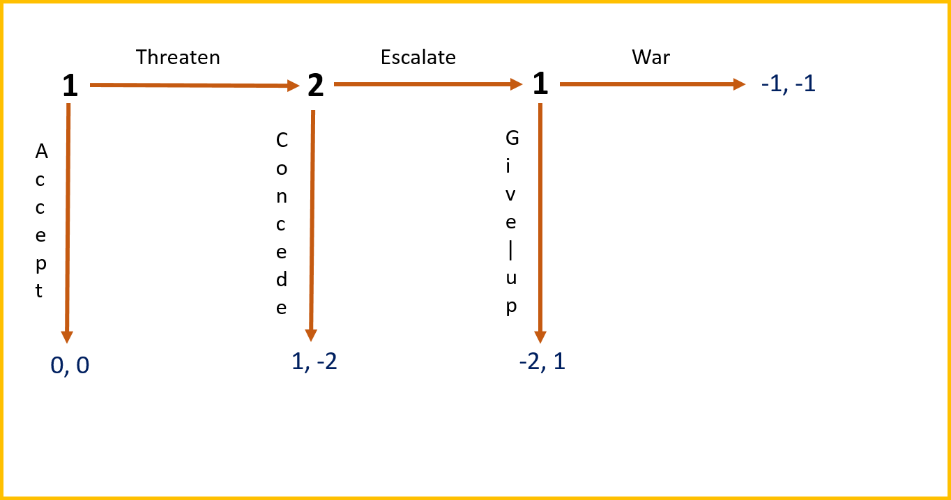
There are two players in this game—Player 1 and Player 2. In the first stage, Player 1 decides whether to “Threaten” Player 2 or “Accept.” If Player 1 accepts, the game ends with both Players 1 and 2 receiving payouts of $0 each (the number to the left of the comma denotes Player 1’s payout, and the number to the right denotes Player 2’s). If Player 1 chooses to threaten Player 2 in the first stage, then the game proceeds to the second stage where Player 2 gets to choose whether to “Escalate” or “Concede.” If Player 2 concedes, the game ends with Player 1 receiving a payout of $1, and Player 2 is required to make a payment to the experimenter of $2. If Player 2 chooses to escalate in the second stage, then the game proceeds to the third and final stage where Player 1 gets to choose “War” or to “Give up.” If Player 1 chooses Give up, then the game ends with Player 1 making a payment of $2 to the experimenter and Player 1 receiving a payout of $1. If Player 1 instead chooses War, then the game ends with both players required to pay the experimenter $1 each.[9]
Can you guess the logic behind the game’s analytical equilibrium?
Via backward induction, we start at the third and final stage and work our way back to the first stage. We see that Player 1 will declare “war” if the game ever reaches its final stage since paying $1 is a better outcome for Player 1 than paying $2. Knowing this, Player 2 will choose to “escalate” in the penultimate stage since she will be required to pay $1 as a consequence of war occurring in the final stage, which is a better outcome for Player 2 than paying $2. But then knowing this, Player 1 will choose to “accept” in the first period, which leads to a zero payout, which is, nevertheless, a better outcome than the payment of $1 Player 1 would be required to pay as a result of later going to war with Player 2. This is the game’s unique SPE.
Note that in the case of international relations, this game captures the essence of “mutual deterrence.” What drives mutual deterrence in the context of this game is that Player 2 choosing to escalate in the penultimate stage acts as a credible threat to Player 1.[10] What’s the outcome when you and your classmates play this game? Hopefully, you choose mutual deterrence as opposed to going to war.
Escalation Game with Incomplete Information
Spaniel (2011) proposes a tweak to the Escalation Game by endowing Player 1 with less information than Player 2. We assume that Player 1 does not know for certain whether Player 2 is a “weak” or “strong” type. Player 1 therefore assigns probability to Player 2 being weak and  to Player 2 being strong. “Nature” has pre-assigned Player 2 his type, which Player 2 alone is aware of with certainty. Player 1 moves first. When he moves, Player 2 knows both his type and the move made by Player 1 in the first stage.[11] The decision tree for this game looks like this:
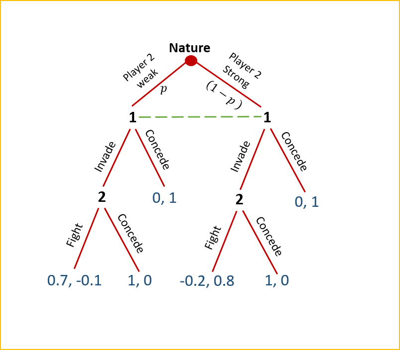
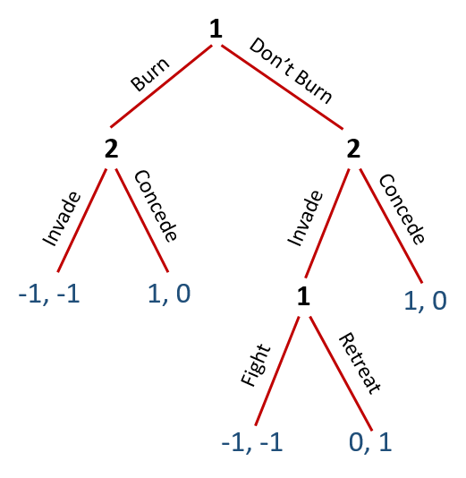
In the initial stage (which we will call Stage 0), Nature determines whether Player 2 is weak or strong. Player 1 assumes Player 2 will be weak with probability and strong with probability , where  . As indicated by the green hashed line, when Player 1 moves in the first stage, she does not know for certain whether Player 2 has been determined as weak or strong. If it turns out that Player 2 was determined by Nature to be weak and Player 1 “concedes,” the game ends with Player 1 receiving a payoff of $0 and Player 2 receiving a payoff of $1. If, on the other hand, Player 1 chooses to “invade,” then Player 2 chooses between “fight” and “concede” in the second stage, resulting in payoffs of $0.70 and -$0.01 and $1 and $0, respectively for Players 1 and 2. If, instead, it turns out that Player 2 was determined by Nature to be strong and Player 1 chooses to concede in the first stage, the game ends with Player 1 again receiving a payoff of $0 and Player 2 receiving a payoff of $1. If Player 1 chooses to invade, then again, Player 2 chooses between “fight” and “concede” in the second stage resulting in payoffs of -$0.20 and -$0.08 and $1 and $0, respectively to Players 1 and 2. Whew!
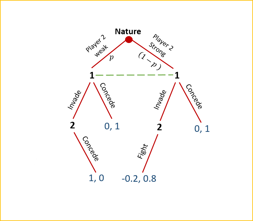
Before working through the logic of the analytical equilibrium, notice that if and when the players reach the game’s second stage, Player 2 will never choose to fight if he was determined by Nature to be weak (remember that Player 2 knows for certain whether he is weak or strong before play begins with Player 1). This is because the payoff from conceding at that stage is $0, which is larger than the payoff of -$0.1 associated with choosing to fight. Similarly, if Player 2 was determined by Nature to be strong, then he will never choose to concede if and when the players reach Stage 2 ($0.8 > $0). Thus, the decision tree for this game can now be depicted as the following:
Now, how do we solve for the game’s analytical equilibrium?[12]
Here, Player 2 applies backward induction to find what’s known as a Perfect Bayesian Equilibrium (PBE). As we already know, if Player 2 is the weak type and Player 1 has chosen to invade, then Player 2 should concede. If he is the strong type, then Player 2 should fight. We also know that Player 1 recognizes that she gets a payoff of $0 if she concedes in the first round, regardless of Player 2’s type. If she instead chooses to invade in the first round, then Player 1’s expected payoff from invading is  . This is merely the weighted average of Player 1’s expected payoff when Player 2 is weak and her expected payoff when Player 2 is strong. Thus, invade is a better strategy than concede for Player 1 when
  . In other words, if the probability that Player 1 assigns to Player 2 being weak is greater than one-sixth, Player 1 should choose to invade in the first round. Otherwise, Player 1 should concede and be done with it.
What’s the outcome when you and your classmates play this more complicated version of the Escalation Game?
Burning Bridges Game
This game shares starkly similar features with the Escalation Game, but there is no uncertainty (thus, the analytical equilibrium is an SPE rather than a PBE). The SPE has much to say about the relationship between two tenacious competitors. Spaniel (2011) portrays the game as follows:
Suppose an island is located between two countries. Each country has a bridge to the island.
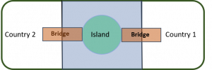
Country 1 decides to cross over its bridge to the island in an act of war. Country 1 must then choose whether to burn the bridge behind it or not.
The game’s structure is depicted by the following decision tree:
Recall that this game starts with Country 1 already having crossed the bridge onto the island. Country 1’s choice in the first stage of the game is, therefore, whether or not to burn the bridge behind it. If Country 1 burns the bridge, then Country 2 must decide whether to cross its bridge and invade the island as well or to concede the island to Country 1. The resulting payoffs for the two countries are as shown. If, instead, Country 1 chooses not to burn its bridge, then if Country 2 also decides to invade the island, Country 1 must then choose whether to stand and fight or retreat back over its bridge to safety. Otherwise, if Country 2 decides to concede, then the result is the same as when Country 1 decides to burn its bridge.
The logic for the analytical equilibrium goes like this:
If Country 1 chooses not to burn its bridge, Country 2 will choose to invade the island knowing that Country 1 will then choose to retreat (since $0 > -$1), thus giving Country 2 a payoff of $1, which is larger than the payoff it would have gotten had it instead chosen to concede. Thus, Country 1’s payoff from choosing not to burn its bridge is ultimately $0. If Country 1 instead chooses to burn its bridge, Country 2 will choose to concede (since $0 > -$1), giving Country 1 a payoff of $1. Thus, Country 1 choosing to burn its bridge and Country 2 responding by conceding the island to Country 1 is this game’s SPE.
There are historical examples of this game having been played between civilizations and countries and even individuals. For example, Collins (1989) recounts an incident in 711 AD when Muslim forces invaded the Iberian Peninsula, and commander Tariq bin Ziyad ordered his ships to be burned, thus signaling to his troops that they had passed the point of no return. Harvey (1925) recounts a similar incident in Myanmar (formerly Burma). In the Battle of Naungyo, during the Toungoo-Hanthawaddy War in 1538, the Toungoo armies led by commander Kyawhtin Nawrahta (later known as Bayinnaung) faced the superior force of Hanthawaddy on the other side of a river. After crossing the river on a makeshift bridge, Bayinnaung ordered the bridge to be destroyed. Similar to Muslim commander bin Ziyad, Bayinnaung took this action to spur his troops forward in battle and provide a clear signal that there would be no retreat. In both cases, the commanders were victorious.
Have you ever burned your proverbial bridge in negotiations with an employer, a friend, or maybe even a family member? If the answer is “yes,” chances are you are not alone. Most Homo sapiens, if they live long enough, are eventually confronted with having to play a game like this. Typically, it requires a curious mixture of courage and desperation for a player (in our case a Country 1) to summon the will necessary to achieve the game’s analytical equilibrium.
Police Search
Spaniel (2011) describes a game he once remembers having played himself. The title of the game says it all:
Suppose a police officer pulls Big Al over and asks to search his vehicle. Big Al can let the police officer search the vehicle (which could be a quick or a thorough search, depending upon the police officer’s preferences) or refuse and force the officer to call in the Canine Unit. Big Al’s preferences are Quick Search  Canine Unit Thorough Search, while the police officer’s preferences are Quick Search Thorough Search Canine Unit.
Without actually knowing Big Al’s preferences, the officer nevertheless claims that “a Quick Search is more preferred for both of us than calling in the Canine Unit.”
Recall from Chapter 3 that the symbol stands for “strictly preferred to.” Thus, we can say that based upon the information given above, Big Al strictly prefers a quick search as opposed to summoning the canine unit, and strictly prefers the canine unit as opposed to a thorough search. In contrast, the police officer strictly prefers the thorough search over a quick search, and strictly prefers the quick search over bringing in the canine unit.
It helps if this game is depicted as a decision tree.
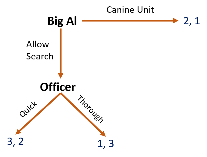
Note that the hypothetical payoffs associated with each choice in the decision tree correspond with Big Al’s and the police officer’s respective preference rankings. To find this game’s analytical equilibrium, we need to assume common knowledge among Big Al and the officer (i.e., each player knows both his own payoffs and those of the other player). Common knowledge has been implicitly assumed for each of the games examined thus far except, of course, in the case of the Escalation Game with Incomplete Information. The logic for the analytical equilibrium is as follows:
If Big Al allows a search, the officer will choose to do a thorough search, implying Big Al’s payoff is 1 and the officer’s is 3. If, instead, Big Al does not allow the search, the Canine Unit is called in, resulting in payoffs to Big Al and the officer of 2 and 1, respectively. Clearly, the game’s SPE is Big Al not allowing a search, and the officer calling in the canine unit.
In some sense, by holding his ground on not allowing the officer to search his car, Big Al is burning his bridge with the officer. The equilibrium outcome is driven by the fact that the officer cannot credibly commit to conducting a quick search if Big Al were to allow the officer to conduct a search. Sadly, the resulting SPE for this game is inefficient since, as the officer originally pointed out, both Big Al and the officer prefer the quick search. If Big Al and the officer were Homo economicus rather than Homo sapiens, they would mutually trust each other in this particular context, and the quick search would be conducted. Both the officer and Big Al would save valuable time, and the canine unit would get more rest.
Two-Stage Iterated Dominance Game
Beard and Beil (1994) propose the following game:
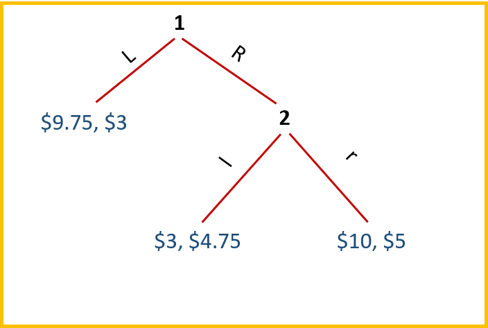
Player 1 chooses first, moving either left (L) or right (R). If she moves L, the game ends with Players 1 and 2 receiving payouts of $9.75 and $3, respectively. If, instead, Player 1 moves R, then Player 2 chooses in the second stage whether to move left (l) or right (r). The payoffs to both players are then as given. The game’s SPE is determined via the following logic:
By backward induction, Player 1 considers what Player 2 will choose if the game proceeds to the second stage. Player 2 will choose r since $5 > $4.75. This results in $10 for Player 1, which is larger than the $9.75 payout she would obtain if she decides to move L in the first stage. Thus, Player 1 choosing R and Player 2 choosing r is the game’s SPE (denoted (R,r)).
After playing this game with various groups of Homo sapiens, Beard and Beil (1994) report that 66% of Player 1s chose to move L.[13] In the 34% of instances where Player 1s moved R, their choices were met with Player 2’s self-interested response of r 83% of the time. Beard and Beil calculated Player 1’s faith in Player 2’s rationality required to justify choosing R in the first stage (which they label a threshold probability  as equaling 0.97. In other words, Player 1s reported needing to believe that Player 2 would choose r in the second stage 97% of the time before they could justify choosing R in the first stage. Since Player 2s chose r only 83% of the time, the threshold was not quite met on average.
Dirty Faces
Littlewood (1953) invented this iterated-knowledge game whereby three ladies, A, B, and C, in a railway carriage all have dirty faces and are all laughing. Because none of the ladies can see their own face to know for certain whether their face is dirty, they must infer from the laughter of the other two ladies whether their own face is dirty. The version of this game presented in Camerer (2003) involves only two players, but the notion of iterated knowledge is nonetheless retained.
Two players have independently and randomly drawn their “types”, either X or O, with probabilities of 80% and 20%, respectively. After observing the other player’s type—but not their own type—the two players choose either “Up” or “Down.” Payoffs for each player are given in the matrix below.
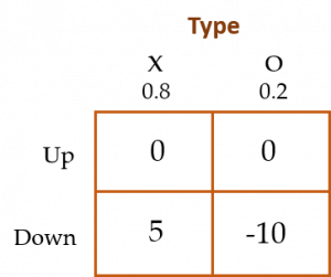
Thus, if a player chooses Up, he earns nothing. If a player chooses Down, he earns $5 if he is type X and loses $10 if he is type O. When at least one player is type X, both players are told, “At least one player is type X.” Successive rounds of the game are played (with each player retaining their original type) until one of the players chooses Down. After each round, the players are told of the other player’s choice.
The logic for the analytical equilibrium goes like this:
There are two cases to consider—the XO case (one player is X and the other is O) and XX (both are X). We do not need to consider the OO case since, when this happens, each player will know immediately that he is an O type (how?) and thus, neither of the players will ever choose Down.[14]In the XO case, the player who is X can infer this fact (how?). He then moves Down. In the XX case, both players know there is at least one type X (after the announcement is made that at least one of the players is type X), and they know the other player is X, but they still know nothing for certain about their own type. Each player, therefore, chooses Up in the first round and is then told of the other player’s choice. Player 1, for example, is told that Player 2 chose Up. Player 1, therefore, infers that Player 2 must have known Player 1 was a type X. Otherwise Player 2 would have chosen Down. Thus, Player 1 infers his own type from Player 2’s behavior—he must be an X. Hence, Player 1 chooses Down in the second round. And therefore, for the case of XO, we expect the type X player to choose Down in the first round of the game, while in the case of XX, we expect both players to choose Down in the second round of play (after the first announcement of player choices has been made by the experimenter).
Weber (2001) enlisted a small group of participants to play the Dirty Faces game. Recall that in Round 1, we expect the equilibrium to be (Down, Up) when the players are types X and O, respectively, and (Up, Up) when both players are type X. In Round 2, played only by players who are both X types, we expect the (Down, Down) equilibrium to result. The author found that in the XO case, player pairs behaved like Homo economicus seven out of eight times across two different trials by choosing Down when they were type X. In the trickier XX case, players are predicted to choose (Up, Up) in the first round, followed by (Down, Down) in the second round (after each player is informed of the other player’s choice). In Weber’s experiment, player pairs chose (Up, Up) in the first round 14 out of 18 times. But, only four of the 14 player pairs who chose (Up, Up) in the first round chose (Down, Down) in the second round.
The evidence for Homo sapiens is, therefore, mixed. They seem to mimic Homo economicus in the XO case rather well, but not nearly as well in the XX case.
Trust Game
Consider the following game proposed by Berg et al. (1995):
An Investor has $ which she can keep or invest. Suppose she decides to invest $ and keep $(
 ). The investment of $ earns a return, at a rate of (1 +
  ), and becomes $(1 + ). Another player, the Trustee, must now decide how to share the new amount $(1 + ) with the Investor. Suppose the Trustee decides to keep $
 and thus returns $[(1 + ) – ] to the Investor, resulting in a payoff of $ for the Trustee and $[ – + (1 + ) – ] = $[ – +
  ] for the Investor.
Thus, $ is a measure of trust and $[(1 + ) – ] is a measure of trustworthiness.
For our game, let = $200 and = 1.
Despite the relatively complicated calculations involved in determining the returns to the Investor and Trustee for different possible investment and share values, the logic behind the game’s analytical equilibrium is a straightforward application of iterated dominance practiced by the investor, in particular backward induction.
Because the Investor anticipates that the Trustee will keep whatever investment is made, the Investor chooses to keep the entire $200 and thus invests nothing! Consequently, in this game’s SPE, there is no trust displayed by the Investor and no opportunity for trustworthiness, or “direct reciprocity,” to be displayed by the Trustee.
Not so with Homo sapiens. Berg et al. find that Investors invest roughly 50% on average (i.e.,  = 50%), and Trustees repay roughly 95% of what was invested (i.e.,
  = 95%), which equals a negative return to trust and a correspondingly slight lack of trustworthiness![15] In a modest tweak, Buchan et al. (2000) engage Asian and American subjects in a trust game where the Investor knows she will receive the return from a different (i.e., third-party) Trustee rather than the original Trustee. The authors find that both trust and trustworthiness decrease relative to Berg et al.’s findings (i.e., a sense of karma—that one would hope exists among Trustees—does not restore trust and trustworthiness). Buchan et al.’s (2000) results are contained in the table below.
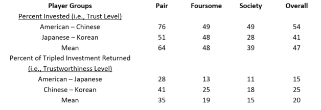
The different groups are similar (e.g., when it comes to Investors, American and Chinese subjects behaved similarly to each other, and Japanese and Korean subjects behaved similarly as well). As Trustees, American and Japanese subjects behaved similarly, and Chinese and Korean subjects behaved similarly. “Pair” represents a control treatment where the Investor receives a return from the same Trustee she invests with. The Foursome treatment refers to a version of the game where there are two Investors (A and B) and two Trustees (C and D). Investor A originally invested with Trustee C but is repaid by Trustee D, and Investor B originally invested with Trustee D but is repaid by Trustee C. Investors A and B know this “cross repayment” is occurring. The Society treatment refers to the case where Investors and Trustees are in separate rooms, and which Trustee repays which Investor is determined randomly. Investors A and B, therefore, do not know which Trustee has been assigned to them ahead of time. The “Overall” column provides the average across these different treatments.
We see that, on average, Investors chose to invest 64% of their initial amount with the Trustee in the control treatment (which exceeds Berg et al.’s finding of 50%). However, alternative pairings of Investors with Trustees lead to a reduction in the investment made by investors (i.e., a decrease in trust). Overall, trust is effectively displayed at a 47% level. Similarly, although in the control treatment 105% of the Investor’s initial investment is returned (35 x 3 = 105%), the overall return on investment is only 60% (20 x 3 = 60%), which represents a markedly lower level of trustworthiness than found by Berg et al (1995).
Carter and Castillo (2011) conducted similar trust experiments with relatively poor and lower-educated residents in rural and urban communities in South Africa. On average, Investors trusted their anonymous partners with 53% of their investable income, remarkably close to the percentages observed in the U.S. experiments performed by Berg et al. (1995). However, the amounts invested varied substantially depending upon which village the Investor was from. Similarly, on average, Trustees reciprocated in a trustworthy manner by returning 100% of the Investor’s investment. Carter and Castillo also found that trust and trustworthiness went hand-in-hand—residents located in villages with higher levels of trust also tended to exhibit higher levels of trustworthiness. Further, in urban communities, higher levels of trust and trustworthiness are correlated with higher levels of household expenditures (a proxy for household well-being), while in rural communities this relationship is reversed—higher levels of trust and trustworthiness are associated with lower levels of household expenditure.
One potential explanation for these latter results is that trust in a rural village is prone to moral hazard (Just, 2013). Moral hazard occurs when a person’s actions are not fully observed by others, yet they can affect the welfare of both that person and others. A trusting rural village might mean that residents generally assume that everyone else will perform their civic and economic duties and therefore do not need to be closely monitored. The marginal gain in household well-being from trusting others a bit more is, therefore, relatively small. In a less-trusting village, residents will monitor each other more closely to learn whether others are actually performing their work, potentially leading to a larger marginal gain in household well-being as a result of being able to trust others more. Alternatively, very few residents in an urban area are related to each other. This means that trusting others more might allow you to build a wider social network, potentially creating some substantial gains in household well-being from being able to trust others more.[16], [17]
Multi-State (“Centipede”) Trust Game
The multi-stage trust game is best represented in the form of a decision tree:
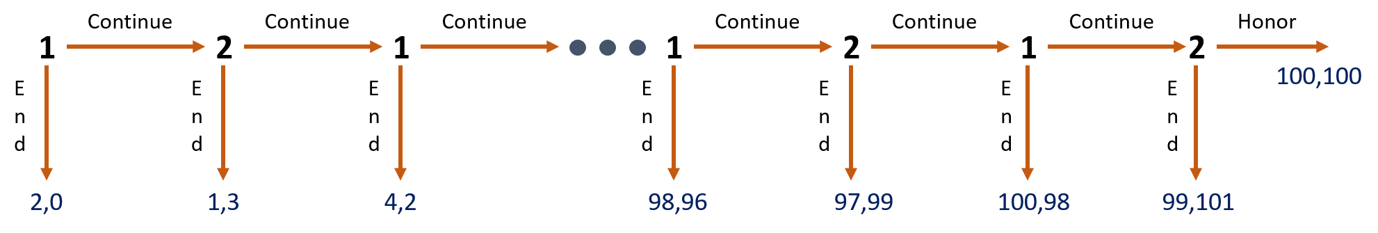
Player 1 acts as the investor in the first stage by choosing whether to end the game immediately by not investing (in which case she obtains a payoff of $2 and Player 2—acting as the Trustee in this stage—gets nothing), or by investing and continuing the game to the second stage. In the second stage, Player 2 now acts as the Investor and decides whether to end the game by not investing (in which case she obtains $3 and Player 1—acting as the Trustee in this round—gets $1), or by investing and continuing the game to the third stage where, once again, Player 1 acts as the Investor and Player 2 the Trustee. As depicted, the game can be played up to 100 stages. And now we see how this game got its moniker—its decision tree bears a striking resemblance to a centipede.
The logic for the analytical equilibrium goes like this:
Via backward induction, Player 2 (as Investor) ends the game in the final stage with no investment (thus earning a payoff of $101). Knowing this will happen, Player 1 (as Investor) ends the game in the penultimate stage with no investment (thus earning a payoff of $100, which is larger than the $99 she would have earned as Trustee had the game instead ended in the final stage). As the game unravels in mistrust all the way back to the first stage, Player 1 (as Investor) chooses to end the game in the first stage with no investment (thus earning a payoff of only $2). This game’s SPE is woefully inefficient. Too bad Homo economicus are so self-interested. Had they been able to cooperate with each other they could have played to the final round, with Player 1 earning $99 and Player 2 earning $101.
Camerer’s (2003) survey of the literature suggests that Homo sapiens tend to reciprocate trust and trustworthiness for a few stages before one of the players ends the game. This may be a case of Player 1 believing Player 2 lacks common sense. Player 1 thus plays Continue in the first stage, sending a signal that she trusts Player 2, who then also chooses Continue in the second stage. In cases where altruistic players are involved, the Honor payoffs in the final period may be interpreted as (101, 102), and the players are self- and dual-motivated to advance all the way to the final stage.
In a novel laboratory experiment, Scharlemann et al. (2001) led participants to believe that they were playing the Centipede game with a randomly paired partner. Before choosing a strategy, Player 1 was given a photograph of the player (Player 2) to whom he was purportedly paired, and likewise for Player 2, who was given a photograph of purported Player 1. In reality, both players were playing against predetermined strategies programmed into a computer. Nevertheless, each player believed he was playing against the player in the picture.
There were actually two pictures of each purported player. One of the photos depicted the player smiling, and the other depicted the player with a straight face. Participants were randomly assigned to see either a smiling or a straight-faced partner. Overall, the authors found that participants were roughly 13% more likely to choose Continue at the first stage when their supposed partner was smiling in the photograph. Thus, there is some evidence to suggest that participants interpreted a smile on their partner’s face as signaling trustworthiness.
Further, this “smile effect” was noticeably larger for male participants than for female participants. Male participants trusted a smiling partner roughly 20% more than a non-smiling partner, while female participants trusted smiling partners only 6% more. Additional experiments by the authors using other facial expressions also had an impact on the willingness of participants to trust each other.
As the saying goes, what’s in a smile? Perhaps the trust it inspires in those who are graced by one.
To wrap up our exploration of the centipede game, consider McKelvey and Palfrey’s (1992) version where, rather than the payoffs associated with successive stages of the game alternating between increases and decreases (as depicted in the game above), the payoffs increase at a constant rate for both players. Note that investigating possible effects associated with changes in the way payoffs evolve in the centipede game is reminiscent of investigations into the effects of changing the payoffs (or stakes) in the Ultimatum Bargaining and Beauty Contest games discussed earlier (recall that changing the stakes in these two games generally had no impact on the games’ respective outcomes in experiments with Homo sapiens).
In their laboratory games, McKelvey and Palfrey start with a total pot of $0.50 divided into two smaller pots of $0.40 and $0.10. Each time a player chooses to “pass” (i.e., continue), both pots of money are multiplied by two. The authors construct both a two-round (four-move) and a three-round (six-move) version of the game. McKelvey and Palfrey also consider a version of the four-move game in which all payoffs are quadrupled. The authors found that, as with the traditional centipede game described above, the SPEs for these two versions of the game are for Player 1 to “take” (i.e. end) the games in the first round.
In each experimental session, McKelvey and Palfrey use a total of twenty subjects, none of whom had previously played a centipede game. The subjects (students from Pasadena Community College and the California Institute of Technology), were divided into two groups at the beginning of the session, called the Red and Blue groups. In each game, the Red player was the first mover, and the Blue player was the second mover. Each subject then participated in ten games, one with each of the subjects in the other group. Subjects did not communicate with each other except through the choices they made during the game. Before each game, each subject was matched with another subject of the opposite color with whom they had not yet been previously matched. The paired subjects then played either the four-move or six-move game.
McKelvey and Palfrey found that in only 7% of the four-move games, 1% of the six-move games, and 15% of the high-payoff four-move games did Player 1 choose “take” in the first round. The subjects do not iteratively eliminate dominated strategies as they would if, like Homo economicus, they played SPE strategies.[18] In each of the sessions, the probability of a player choosing “take” increases as they get closer to the game’s last move. Thus, as subjects gain more experience with the game, their behavior mimics that of Homo economicus.
Study Questions
Note: Questions marked with a “†” are adopted from Just (2013), those marked with a “‡” are adopted from Cartwright (2014), and those marked with a “ ” are adopted from Dixit and Nalebuff (1991).
- Recall the Ultimatum Bargaining game studied in this chapter. A Proposer makes an initial offer to a Responder of how to split $100. If the Responder accepts the Proposer’s offer, the $100 is split accordingly. If the Responder rejects the Proposer’s offer then both receive $0. As we showed, the analytical equilibrium for this game is the Responder offering $0.01 and the Responder accepting. How would the analytical equilibrium for this game change if the game instead adhered to the following rules: In the first stage, the Proposer makes an offer to the Responder of how to split the $100. In the second stage, the Responder can choose to either accept the offer as is, or agree to a flip of a fair coin. If the coin comes up “Heads,” then the game moves to the third stage. If the coin comes up “Tails,” the game ends with Proposer and Responder each receiving $0. In the third stage, the Proposer can decide to either split the $100 50%-50% (i.e., give $50 to the Responder and keep the remaining $50), or agree to a flip of a fair coin. If the coin comes up “Heads,” the Proposer keeps $75 and gives the Responder $25. If the coin comes up tails, the Proposer instead gives the Responder $75 and keeps $25. What is the analytical equilibrium for this version of the Ultimatum Bargaining game? Explain.
- Knowing what you know about basins of attraction, or path dependence, explain your strategy for playing repeated rounds of the Continental Divide game.
- What would the analytical equilibrium of the Beauty Contest game be if factor were instead set equal to a number greater than 1, say, 1.4? Show how you arrive at your answer.
- Recall the Traveler’s Dilemma game where two travelers simultaneously submit claims to the airline for their lost luggage ranging between $300 and $750. The airline pays both travelers the minimum claim, and then subtracts $50 from that amount for the player who submitted the higher of the two bids and adds $50 to that amount for the player who submitted the minimum of the two bids. In comparison with the analytical equilibrium for this game, explain why the airline should expect to pay out more in claims to two Homo economicus travelers and less in claims to two Homo sapiens travelers if it changed the game accordingly: The travelers get to choose one of two options. Option 1 is the same as the original game, except now the lower-bound on the range of claims is $250 instead of $300. For Option 2, the airline flips a fair coin. If the coin comes up “Heads,” the traveler receives $750; if it comes up “Tails,” the traveler receives $0.
- Calculate the Perfect Bayesian Equilibrium (PBE) for the Burning Bridges game if Country 2 is uncertain as to whether Country 1 has burned its bridge after it (Country 1) has occupied the island.
- † Suppose you are a bank manager. You know that if depositors trust your bank, they will be willing to accept a lower interest rate on deposits. (a) Given what we know of how people develop trust, what might you do to enhance your depositors’ trust? (b) What steps might you take to ensure that your loan officers can avoid potential pitfalls when it comes to originating loans to business owners and other customers?
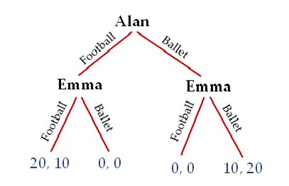
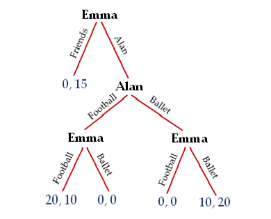
- ‡ Suppose Alan and Emma are locked in a sequential-move version of the Battle of The Sexes game depicted below (you will be introduced to the classic simultaneous move version of this game in Chapter 8). Alan chooses first, choosing to attend either the football game or ballet. Next, Emma chooses the football game or the ballet. The first value(s) at each terminal node of the decision tree represents the payoff(s) accruing to Alan, and the second value(s) represents the payoff(s) accruing to Emma (all in dollars). What is the most likely outcome of this game? Discuss how you have arrived at your answer.
- ‡ Now suppose that in her sequential Battle-of-The-Sexes game with Alan, Emma has an outside option that comes into play at the outset. She chooses to either go out with her friends or “throw her lot” in with Alan for either the football game or ballet. What is the most likely outcome of the game now? Again, discuss how you have arrived at your answer.
- Choose a sequential game you learned about in this chapter. In what way might permitting communication between the players before the game begins affect the game’s outcome?
- Consumers who choose to purchase used vehicles from used-vehicle salespeople complain that the bargaining process resembles an ultimatum bargaining game. Why might this be the case?
- In the game of roulette, betting is based on where a ball will land when a spinning wheel stops. In the game’s simplest form, there are numbers zero through 36 on the wheel. When the ball lands on zero, the players win nothing (or, alternatively stated, the “house” wins). The safest bet in roulette is simply to bet that the wheel will stop on an even or odd number, with numbers zero through 36 on the wheel the chances of winning are 18/37, or a little less than 49%. This bet pays “even money” (i.e., a $1 bet returns $1, leaving the player with a total of $2). A second possible bet would be that the wheel will stop spinning on a multiple of three (e.g., the numbers 3, 6, 9, etc.) for a 12/37, or slightly larger than a 32% chance of winning. This bet pays “two-to-one” (i.e., a $1 bet returns $2 for a total of $3). When players place their bets ahead of the spin of the wheel, they inevitably do so sequentially – no rule says they must place their bets simultaneously with the spin of the wheel or with each other. Whenever a player bets wrong, e.g., places an even-money bet on an odd number and the wheel stops on an even number, or vice-versa, the player loses whatever amount of money was placed on the bet. Suppose that in this game the only possible bets are (1) the even-money bet on an even or odd number, or (2) the two-to-one bet on a multiple of three. Bonnie and Clyde are down to the last spin of the wheel. Whoever has amassed the most money (in terms of the value of their chips) at end of the final spin buys dinner. Bonnie has $700 worth of chips and Clyde has only $300. All else equal, what is Clyde’s best bet? What is Bonnie’s best bet? Does either player have a first-mover advantage?
- Suppose a new store called Newbies is considering entering a market that is currently dominated by a store called Oldies (i.e., Oldies is currently a monopoly in this market, earning $200,000). It is common knowledge that if Newbies enters the market and Oldies accommodates (i.e., does not wage a price war), Newbies will earn $100,000 and Oldies will also earn $100,000. If Oldies instead chooses to launch a price war, then Newbies will ultimately lose $200,000 and Oldies will lose $100,000. Draw the decision tree for this game and determine its subgame equilibrium.
- Suppose the state of Utah institutes a new statewide program called the Utah Brigades, which requires every high school senior to register for a year of public service to the state upon graduation. Worried that this new requirement may lead to mass civil unrest among the students, and unwilling to punish each student who refuses to register, the state announces it will go after evaders in alphabetical order by last name. (a) Explain why this approach could lead to full compliance with the registration. (b) Would this approach still work if the state announced it will go after evaders by Social Security Number, in either ascending or descending order?
- Suppose two parents would like their adult children to communicate with them on a more regular basis. They announce a new quota that each respective child must meet in order to receive their portion of the parents’ inheritance: one visit and two phone calls per week. Any child who does not meet the quota on any given week is disinherited, and the remaining children split the inheritance among themselves. Recognizing that their parents are very unlikely to disinherit all of them, the children get together and agree to cut back on their visits and phone calls, potentially down to zero. What change could the parents make to their will to ensure that the children meet their quota?
Media Attributions
- Continental Divide Matrix © Van Huyck et al.; 1997 Elsevier Science B.V. is licensed under a All Rights Reserved license
- Figure 7 (Chapter 7) © Arthur Caplan is licensed under a CC BY (Attribution) license
- Figure 8 (Chapter 7) © Arthur Caplan is licensed under a CC BY (Attribution) license
- Figure 9 (Chapter 7) © Arthur Caplan is licensed under a CC BY (Attribution) license
- Burning Bridges Figure © Arthur Caplan is licensed under a CC BY (Attribution) license
- Figure 11 (Chapter 7) © Arthur Caplan is licensed under a CC BY (Attribution) license
- Figure 13 (Chapter 7) © Arthur Caplan is licensed under a CC BY (Attribution) license
- Figure 14 (Chapter 7) © Arthur Caplan is licensed under a CC BY (Attribution) license
- Dirty Faces Figure © Arthur Caplan is licensed under a CC BY (Attribution) license
- Table 1a (Chapter 7) © Colin F. Camerer; Princeton University Press is licensed under a All Rights Reserved license
- Figure 17 (Chapter 7) © Arthur Caplan is licensed under a CC BY (Attribution) license
- Figure for Study Question 8 (Chapter 7) © Arthur Caplan is licensed under a CC BY (Attribution) license
- Figure for Study Question 9 (Chapter 7) © Arthur Caplan is licensed under a CC BY (Attribution) license
- The Nash equilibrium solution concept is attributed to John Nash Jr., an American mathematician and the winner of the 1994 Nobel Memorial Prize in Economic Sciences. Nash published his pioneering work in non-cooperative game theory in the early 1950s (Nash, 1950a, 1950b, 1951). His struggles with mental illness and recovery are recounted in Sylvia Nasar’s 1998 biography A Beautiful Mind and later, the 2001 film of the same name. ↵
- Just (2014, pages 420-422) provides a mathematical framework within which to assess the same outcomes of this game as we demonstrate here with more intuitive game-theoretic reasoning. ↵
- An extreme form of Ultimatum Bargaining is known as the Dictator Game, whereby the Proposer makes an offer that the Responder must accept (i.e., the Responder is not allowed to reject). There is no iteration and no real role or advantage for having information. Yet, there is a dominant strategy for the Proposer, which results in an analytical equilibrium where the Proposer offers nothing to the Responder (i.e., = 0) and the Responder accepts. Obviously, in this game, “Responder” is a euphemism for “Lackey.” See Forsyth et al. (1994), Hoffman et al. (1994), Hoffman et al. (1996), and Fehr and Fischbacher (2004) for experiments with the Dictator Game. ↵
- Technically speaking, a subgame perfect equilibrium is obtained when a Nash equilibrium has been reached at every subgame of the original game, even if a particular subgame has not been played. In the case of Ultimatum Bargaining, there are two subgames: one where the Responder either accepts or rejects the offer, and the other is the full game itself (the full game is always considered a subgame). We will learn more about what defines a “subgame” a bit later in the chapter. ↵
- Gladwell (2002) recounts a classic example of path dependence—The Broken Window Theory. The theory is that a single broken window left unfixed in a neighborhood can lead to a spiraling process of social breakdown as those with criminal intent interpret the broken window as a signal that the neighborhood is in decline and thus less able to protect itself. The broken window sets the neighborhood on the path toward a low Nash equilibrium. ↵
- Keynes (1936) described the action of rational agents in an equity market using the analogy of a fictional newspaper contest where participants were instructed to choose the six most attractive faces from among a hundred photographs. Those who chose the most popular faces were then eligible for a prize. ↵
- Note that this is a game where backward induction is again moot, and the only subgame is the game itself. ↵
- Decision trees in game theory are known as games depicted in “extensive form.” Drawing a decision tree is typically the most effective way to depict a multi-stage game. ↵
- Note that depicting the game in extensive form makes it easy to identify the number of different subgames. In this case there are four subgames. ↵
- Here’s a test to see how well you’ve grasped the logic behind the game’s analytical equilibrium. What equilibrium would result if instead of having to pay $2 by choosing to “concede” in the second stage, Player 2’s required payment was instead something less than $1? ↵
- This type of game is also known as a “screening game,” where the lesser-informed player moves first. ↵
- This equilibrium is known as a Perfect Bayesian Equilibrium (PBE) rather than an SPE because of the uncertainty that at least one of the players is forced to contend with. Similar to Nash, Thomas Bayes is considered a towering figure. He was an 18th-century English statistician, philosopher, and Presbyterian minister who is known for formulating a specific case of the theorem that bears his name: Bayes Theorem. Bayes never published his theory himself—his notes were edited and published posthumously. ↵
- These results are for Beard and Beil’s (1994) baseline treatment. The authors considered several other treatments where the payoffs for the two players were modified. The results for most of these alternative treatments were qualitatively similar to those obtained in the baseline treatment. ↵
- In actual experiments conducted by Weber (2001) with Homo sapiens, results for cases where both players drew the O type are left unreported. ↵
- The threshold for displaying trustworthiness in this game is 100% of the Investor’s investment returned by the Trustee. ↵
- Stanley et al. (2011) conducted trust games in the US with participants of different races and found that differences in trust and trustworthiness can be partially explained by differences in implicit attitudes toward race. Similar differences in trust and trustworthiness between races were discovered in earlier experiments conducted by Glaeser et al. (2000). In their laboratory experiments, Johansson-Stenman et al. (2009) find weak differences in trust and trustworthiness among Bangladeshi individuals with different religious identities (Hindu and Muslim). Croson and Buchan (1999) find no significant effect of gender on Investors’ level of trust. However, the authors find that women Trustees reciprocate significantly more of their wealth in trust games than men, both in the US and internationally. In a novel laboratory experiment, DeBruine (2002) finds that trust game participants were more likely to trust others who look more like they do, which suggests that people over generations evolve toward promoting the well-being and survival of others with whom they share a resemblance. ↵
- Carter and Castillo (2004) conducted a trust experiment with survivors of Hurricane Mitch, which devastated rural Honduran communities in 1998, with the goal of measuring the extent to which trust among community members helped spur recovery efforts. As the authors point out, while many communities received some inflow of external aid, the absence of insurance contracts and thinness of capital markets meant that most households had to rely either on their own resources to muster an economic recovery, or on resources that they could broker through social relationships. Econometric analysis of the experimental data provided evidence of durable community norms, such as trust that is reinforced by social interactions. The analysis shows that trust played a strong, but uneven role in facilitating recovery from Hurricane Mitch, assisting most strongly a favored subset of households. While establishing the importance of norms such as trust, Carter and Castillo’s analysis warns against the presumption that all community members are equally well-served by the social mechanism of trust in the face of recovery from a natural disaster. ↵
- Instead, the players exhibit what on the surface appears to be altruistic behavior. However, as McKelvey and Palfrey point out, if a selfish player believes that there is some likelihood that each of the other players may be altruistic, then it can pay the selfish player to mimic the behavior of an altruist in an attempt to develop a reputation for choosing to “pass.” The authors surmise that the incentives to mimic are very powerful, in the sense that a very small belief that altruists are in the subject pool can generate a lot of mimicking, even when the players face a very short time horizon. McKelvey and Palfrey ultimately estimate that their sample consists of only 5% altruists. ↵
