As mentioned previously, this chapter presents additional laboratory experiments designed to test the implications of the theories advanced in Chapter 4. Here, we learn about the classic advances made by behavioral economists and the main concepts underscored by Prospect Theory; concepts such as mental accounting, Ambiguity and Competency Effects, fairness, regret and blame, as well as loss aversion, reference dependence, and the Endowment Effect.

Mental Accounting (Version 1)

Consider the following two experiments proposed by Kahneman and Tversky (1984):

Homo economicus would recognize that, regardless of whether he had the $10 ticket in hand but lost it or lost $10 in cash beforehand, once at the cinema the $10 reduction in his income is what’s known as a “sunk cost.” He would therefore ignore this cost—completely put it out of his mind—and instead answer the question, “Is watching this movie worth $10 to me at this moment?” If the answer is “yes,” then he purchases the ticket and watches the movie. If the answer is “no,” he heads back home and does not watch the movie. Most importantly, Homo economicus’ answer to the question is not dependent on whether he lost the ticket itself (as in Experiment 1) or the cash (as in Experiment 2) (i.e., Homo economicus would not be guilty of “narrowly framing” his answer on whether it was a ticket or cash that was lost). As a result, we would expect the percentage of Homo economicus choosing to pay for another ticket in each experiment to be roughly 50%.

Based on samples of roughly 200 subjects each for two similar experiments, Kahneman and Tversky found that 46% of the subjects in Experiment 1 answered “yes,” they would pay $10 at the box office for another ticket, while in Experiment 2, 88% answered “yes.”  The authors conclude that going to the cinema is normally viewed as a transaction in which the cost of the ticket is exchanged for the experience of seeing the movie. Buying a second ticket increases the cost of seeing the movie to a level that many Homo sapiens find unacceptable. In contrast, the loss of cash is not posted to the mental account of the movie, and it affects the purchase of a ticket only by making the individual feel slightly less affluent.^[1]

This evidence suggests that Homo sapiens is prone to mental accounting while Homo economicus is not.

A Homo economicus participating in Experiment 1 would recognize the same thing as a Homo economicus participating in Experiment 2—he saves $15 by making the trip to the other store. Further, we can say that Homo economicus would not distinguish between $15 saved on a relatively cheap vs. expensive pair of earbuds, and thus, we would expect 50% of the Homo economicus in each experiment to choose to make the trip to the other store. All else equal, we should expect the full cost of traveling to the other store to exceed the $15 savings for half of the Homo economicus who would therefore choose not to make the trip.

When it comes to Homo sapiens, Kahneman and Tversky found that 68% of their roughly 100 subjects in Experiment 1 chose to make the trip to the other store, while only 29% of their subjects in Experiment 2 chose to make the trip. This is another example of mental accounting, whereby Homo sapiens relate the savings associated with making the trip to a reference point that is determined by the context in which the decision arises. In this case, a larger percentage of Homo sapiens interpreted the savings on the cheaper pair of earbuds to be worth the trip to the other store. Apparently, saving money on a cheaper pair of earbuds is more valuable than saving the same amount of money on a more expensive pair.

This example relates to what Thaler (1980 and 1985) calls transactional utility, whereby consumers base their purchase decisions on whether they derive value from the belief that they are getting a good deal rather than just the utility derived from the actual item purchased, or what Thaler calls acquisitional utility. The extent to which purchasing decisions are driven by transactional utility helps explain why stores consistently mark certain products as being “on sale.” For example, consumers are more likely to buy a product marked “on sale” for $4 when it regularly sells for $6 than they are to buy the same product simply marked as $4. The product may be for sale at the same price, but consumers feel they are getting a better deal when it is “on sale” than when they pay a regular price.

Could there be a better explanation for these experimental results, perhaps something more conclusive to say about a possible reference point? Looking again at the two experiments, we see that the price differential in Experiment 1 results in a considerably larger percentage gain in savings than the differential in Experiment 2 (specifically, the 50% savings in Experiment 1 is more than double the approximately 20% savings in Experiment 2). Thus, to the extent that Kahneman and Tversky’s subjects based their decisions in this context on percentage savings rather than the actual dollar amount saved, we would expect deviations from Homo economicus’ decision. It may be that several of the experiment’s subjects behaved as if their reference point for making a choice was percentage rather than actual savings.

Mental Accounting (Version 3)

Consider the following experiment:

Because both Patricia and Peter have tickets to see the game, Homo economicus rationalizes that each will simply weigh the expected benefit of braving the blizzard to see the game (which is the psychic joy associated with watching the Jazz compete against the opposing team at the Vivint Center) against the expected cost (the danger of venturing out into the blizzard). Not that this is really germane to the issue at hand (it’s more a nod to the nitpicky among you), but the costs of parking and gasoline to power their vehicles, as well as prorated auto insurance and depreciation of their vehicles and their opportunity costs of the time spent traveling to and from the Vivint Center and watching the game itself are not added to their expected costs because Homo economicus correctly assumes that Patricia and Peter already accounted for those costs when the tickets were purchased and accepted for free, respectively. Regardless, Homo economicus would choose statement C. Those of you who chose statement A suffer from the Sunk Cost Effect. You are mental accountants. There’s no known explanation for those of you who chose statement B.

Similar to the previous experiment with Patricia and Peter, we would expect Homo economicus to pick statement C. When it comes to braving the same snowstorm, it shouldn’t matter who paid when. As Gourville and Soman explain, the timing of Mr. Adam’s and Mr. Baker’s ticket purchases should have no impact on their decision to attend the basketball game. Each should accept that the $40 already spent is a sunk cost and base his decision to go to the game solely upon the perceived incremental costs and benefits of going. Facing the same incremental costs and benefits, Mr. Adam’s and Mr. Baker’s likelihood of attending the game should be equal.

But when it comes to Homo sapiens, all bets are off. Gourville and Soman hypothesize that, in keeping with the prevailing wisdom, both Mr. Adams and Mr. Baker will be prone to the Sunk Cost Effect on purchasing their respective tickets. However, Mr. Adams will have gradually adapted to his “upstream ticket purchase” over the year, thus diminishing the Sunk Cost Effect on his decision of whether to attend the game. The authors call this a Payment Depreciation Effect. To the contrary, Mr. Baker—who has had little time before the game to adapt to the cost of his ticket—will perceive the full Sunk Cost Effect of his purchase when deciding whether to attend. Consequently, Gourville and Soman predict that Mr. Baker will therefore be more likely to attend the game.

The authors test their hypothesis in a series of field experiments with individuals at a shopping mall and laboratory experiments with students. They find support for the Payment Depreciation Effect in a variety of contexts. For example, in a laboratory experiment with over 40 students at the University of Colorado, Gourville and Soman presented the subjects with three tasks spread over three weeks. The first two tasks entailed a short and a long survey, each involving a subject’s evaluation of popular soft drinks. The short survey was designed to require minimal effort and was expected to take approximately five minutes to complete. Thus, in completing the short survey the subject experienced virtually no cost. In contrast, the long survey was designed to require considerable effort and was expected to take approximately 30 minutes to complete. Therefore, completing the long survey exacted a high cost on the subject.

These first two tasks were separated in time by three weeks with the order of the two surveys randomized across subjects—approximately half of the subjects first completed the short survey, then experienced the three-week delay, and then completed the long survey (“no-delay condition” in terms of having incurred the high cost), while the remaining subjects first completed the long survey, then experienced the three-week delay, and then completed the short survey (“delay condition” in terms of having incurred the high cost). Upon completing the second survey, Gourville and Soman paid each subject $7 and then presented the subject with a third and final task—an ostensibly unrelated exercise in which the subject faced a real-money gamble.

The subjects were told they could bet up to $2, in increments of $0.25, on a single roll of a pair of dice. They were told that if they rolled a seven or greater, they would double their bet, but if they rolled a number less than seven, they would lose their bet. They were asked to indicate the amount they were willing to gamble, after which they were asked to roll the dice. Based on the outcome of that roll, the amount they had indicated was either added to or subtracted from their $7 payment they had earlier received for completing the second survey. In keeping with their hypothesis about the Payment Depreciation Effect, the authors expected the subjects in the delay condition to experience less of a Sunk Cost Effect and, therefore, be more likely to gamble more of their $7 payment than subjects in the no-delay condition.

The authors ultimately found that larger numbers of subjects experiencing the delay condition wagered more of their compensation payment on the gamble than subjects experiencing the no-delay condition. The majority of the subjects experiencing the delay condition wagered between $1 and $2, while slightly more than half of the subjects experiencing the no-delay condition wagered between $0 and $1.

Mental Accounting (Version 4)

Consider the following experiments conducted by Prelec and Loewenstein (1998):

When presented with Experiment 1, the authors found that 60% of the roughly 90 participants (visitors to the Phipps Conservatory in Pittsburgh) opted for the earlier payments described in option A despite Prelec and Loewenstein’s estimate of an implicit interest penalty equaling approximately $50 per participant.  However, in Experiment 2, 84% of the same subjects preferred to postpone payments until the washer and dryer arrive (and thus begin paying each month for the next six months after delivery). Thus, Prelec and Loewenstein found that Homo sapiens prefer to decouple payments for durable goods such as washing machines (and thus prorate their payments as their benefits from using the goods occur over time), but not necessarily for goods such as vacations, whose benefits do not extend over time (fond memories of the experience notwithstanding).^[2] This suggests that Homo sapiens fine-tune their mental accounts according to the type of good in question.

As the authors point out, since options A and options B are the same across Experiments 1 and 2 in terms of payment levels and delivery times, we would expect to see no systemic differences in responses from Homo economicus participants across the two experiments. When it comes to Homo sapiens, however, Loewenstein and Prelec find that a higher percentage of the 85 students who participated in the two experiments opted for the lower discount (i.e., greater earlier payment) represented by option A of Experiment 1—where the question is framed as a loss (i.e., a payment)—rather than as a gain (i.e., a rebate) as in option A of Experiment 2. Specifically, 54% of the subjects participating in Experiment 1 stated a preference for option A over B. However, only 33% of the subjects preferred option A over B in Experiment 2.

To explain these results, the authors argue that in Experiment 1 subjects discount future payments less (i.e., future payments loom larger in a subject’s mind), which leads subjects to base their choice upon the size of the total payment—option A’s total payment of $270 is less than option B’s total payment of $275. In Experiment 2, however, the outcomes are framed as gains and are smaller in magnitude, both of which contribute to relatively high discounting of the rebates received in the future, leading to a preference for option B which offers a greater initial rebate. Hence, when it comes to discounting the future, Homo sapiens’ choices are influenced by context, in this case, whether options are framed as future payments due or future rebates to be received. As we well know, Homo economicus is not swayed by this type of framing.^[3]

Overweighting Improbable Events

Consider the following two experiments proposed by Kahneman (2011):

Ok, you know the drill. Let’s start with what Homo economicus would do here. She would calculate the expected payoffs from the two lotteries in each experiment and choose accordingly. Hence in Experiment 1, Lottery B would certainly be chosen since ($5,000 x 1) = $5,000 > ($50,000 x 0.00001) = $0.5, and in Experiment 2, Lottery A would be chosen since (-$50,000 x 0.00001) = -$0.5 > (-$5,000 x 1) = -$5,000. Kahneman reports that in an experiment with roughly 100 subjects, 72% chose Lottery A in Experiment 1 and 83% chose Lottery B in Experiment 2—a marked deviation from what we expect of omniscient Homo economicus.

The results from Experiment 1 highlight Homo sapiens’ proclivity to gamble, while the results from Experiment 2 suggest why we tend to purchase insurance against possible loss. Kahneman and Tversky (1979) go a step further in interpreting these results. They point out that the two experiments demonstrate what they call Possibility and Certainty Effects. On the one hand, lotteries consisting of extremely low probabilities of winning (e.g., 0% – 5%) are still enough to tempt individuals with the possibility of winnings (the Possibility Effect, as demonstrated in Experiment 1). On the other hand, lotteries consisting of extremely high probabilities of losing (e.g., 95% – 100%) are enough to scare individuals into choosing alternatives with lower probabilities, even if those alternatives are associated with high losses (the Certainty Effect, as demonstrated in Experiment 2). As part of their Prospect Theory (discussed earlier in Chapter 4), Kahneman and Tversky point out that Homo sapiens are prone to interpret these extremes as depicting discrete shifts in a lottery’s odds, and thus, the lottery’s expected payoff is essentially ignored. In our minds, we Homo sapiens tend to overweight small probabilities (i.e., improbable events) and underweight moderate and high probabilities (i.e., more likely events).

Based upon their accumulated laboratory experiences over the years, Tversky and Kahneman (1992) eventually proposed decision weights, as shown in the table below (Kahneman, 2011). Recall from Chapter 4 that these weights are derived from a decision-weight formula that effectively transforms a lottery’s objective probabilities of the different outcomes into their corresponding subjective probabilities, or decision weights.

The row of Probabilities represents objective probabilities that could conceivably define a given lottery. The row of Decision Weights represents subjective probabilities that Kahneman and Tversky (1992) suggest we Homo sapiens tend to subconsciously substitute for the objective ones. Note that for lower objective probabilities, the corresponding decision weights are larger (reflecting our penchant for overweighting of improbable events), while for mid- to higher-probabilities, the weights are smaller (reflecting our penchant for underweighting more likely events).

Ambiguity and Competency Effects

Consider the following experiments conducted by Heath and Tversky (1991):

Given that Homo economicus has no particular color preference, he will be indifferent between Lotteries A and B in Experiment 1. This is because the added information provided in Lottery A is superficial in terms of affecting the outcome associated with drawing a marble from the jar. Thus, given any sample of Homo economicus, we would expect 50% to choose Lottery A and 50% to choose Lottery B. In his run of this experiment, Ellsberg (1961) found a larger percentage of Homo sapiens chose Lottery A than Lottery B in what came to be known as the Ellsberg Paradox.  Why? Ellsberg postulates that, although superfluous, the added information provided in Lottery A gives the impression of Lottery A seeming less ambiguous than Lottery B. Thus, Homo sapiens tend to submit to what has also come to be known as an Ambiguity Effect.^[4]

Similarly, in Experiment 2, Homo economicus recognizes that Lotteries A and B are effectively identical. Given the prohibition in Lottery B on one’s ability to check the newspaper or check online, the outcome common to each lottery—the change in a randomly chosen stock’s price—is unaffected by whether the price change occurred yesterday or tomorrow. Thus, given any sample of Homo economicus, we would again expect 50% to choose Lottery A and 50% to choose Lottery B. Lo and behold, in their experiment with roughly 200 subjects, Heath and Tversky found that 67% chose Lottery A. Why?

The authors postulate that Homo sapiens naturally prefer appearing competent or, alternatively stated, prefer not to appear incompetent. By choosing a lottery where the outcome is still to be determined in the future, we perceive ourselves as running less risk of appearing incompetent if the worst outcome occurs (e.g., we guess that the stock price will rise when instead it falls) than if we choose the worst outcome of a lottery where, technically speaking, the outcome has already occurred. In other words, Homo sapiens tend to submit to what has come to be known as a Competency Effect.^[5]

The Decoy Effect

Consider the following experiments proposed by Ariely (2008):

Clearly, all Homo economicus participating in these two experiments who wish to have print versions of The Economist will choose the print-and-internet subscription for $125. It doesn’t matter that the print-only option is missing in Experiment 2. Homo economicus who wish to have print copies of the magazine would never choose that option as long as the print-and-internet option is available. They get more for their money with the print-and-internet option and would therefore never pass it up.

This is what Ariely found for Experiment 1 when 100 of his students at MIT’s Sloan School of Management were presented with the three options. Sixteen students chose the internet-only option and 84 chose the print-and-internet option. No students chose the print-only option. However, when a different group of 100 students participated in Experiment 2, 68 chose the internet-only option and only 32 chose the print-and-internet option. What happened?

As Ariely describes it, this result is the economic equivalent of the theory of relativity; relativity that exposes predictably irrational choice behavior among Homo sapiens. In this particular case, the mere presence of the print-only subscription in Experiment 1 served as a “decoy” that sent 84 of the students to the print-and-internet option. The absence of the decoy in Experiment 2 led the students in that experiment to choose differently. Only 32 students chose the print-and-internet subscription.

This Decoy Effect is a special case of economic relativity. And as Ariely points out, these types of effects mirror the way Homo sapiens’ mind is wired—we are prone to consider things around us in a relative sense. This holds true not only for physical things, such as toasters, bicycles, puppies, restaurant entrées, and spouses but also for experiences such as vacations, educational options, emotions, attitudes, and points of view. Homo economicus, on the other hand, thinks and acts in a world of absolutism.

The Zero-Price Effect

Consider the following two experiments proposed by Shampanier et al. (2007):

Despite having no prior information about the preferences of any given Homo economicus for Lindt truffles vs. Hershey’s kisses, we should nevertheless expect that if 50, 25, and 25 individuals out of a sample of 100 Homo economicus, respectively, were to select the Lindt truffle, Hershey’s kiss, and neither in Experiment 1, then roughly the same respective numbers will be selected by Homo economicus in Experiment 2. Why? Because the difference in prices between the Lindt truffle and Hershey’s kiss is the same in each experiment (50 cents). Rationally speaking, Homo economicus interprets the two experiments as offering the same choice.

To see this, suppose Homo economicus Harry estimates the amount of utility he expects to get from the truffle and the kiss (suppose it’s 150 utils and 50 utils, respectively) and then subtracts the disutility he gets from paying for each. Without loss of generality, suppose each cent paid is a dis-util. In Experiment 1, this means that Harry would receive a net utility (or, net benefit) of 150 – 75 = 75 utils by choosing the truffle, and 50 – 25 = 25 utils by choosing the Hershey’s kiss. Harry therefore gains 75 – 25 = 50 utils by choosing the truffle. In Experiment 2, the net benefit from choosing the truffle is 150 – 50 = 100 utils and the net benefit from choosing the kiss is 50 – 0 = 50 utils. Again, Harry gains 100 – 50 = 50 utils by choosing the truffle. As far as Harry is concerned, the choices in each experiment are identical.

Not so Homo sapiens. Shampanier et al. ran similar experiments with roughly 400 students at the MIT campus and obtained some surprising results. Shampanier et al.’s prices in Experiment 1 were 15 cents for the truffle and 1 cent for the kiss, and in Experiment 2, the prices were 14 cents for the truffle and 0 for the kiss (thus, the choices in each experiment are again identical). To test just how strong the pull of a free Hershey’s kiss might be, the authors had a subgroup of the 400 students instead choose between a 10-cent truffle and a free Hershey’s kiss in Experiment 2.

Shampanier et al. found that 36% of the students chose the Lindt truffle, 14% the Hershey’s kiss, and 50% chose neither in Experiment 1. However, in Experiment 2, only 19% of the students chose the truffle and 42% chose the free kiss. The percentage of students choosing the free kiss was roughly the same (40%) in the version of Experiment 2 where the price of the truffle dropped to 10 cents rather than 14 cents. This “pull” of the free Hershey’s kiss is what Shampanier et al. call the Zero-Price Effect. Apparently, the difference between 15 cents, on the one hand, and 14 or 10 cents on the other is small. But the difference between 1 cent and zero is huge. What gives?

Ariely (2008) puts it this way:

“Most transactions have an upside and a downside, but when something is FREE! we forget the downside. FREE! gives us such an emotional charge that we perceive what is being offered as immensely more valuable than it really is. Why? … it’s because humans are intrinsically afraid of loss. The real allure of FREE! is tied to this fear. There’s no visible possibility of loss when we choose a FREE! item (it’s free). But suppose we choose the item that’s not free. Uh-oh, now there’s a risk of having made a poor decision—the possibility of a loss. And so, given the choice, we go for what is free” (p. 60).

Hmmm. Sounds like a case of loss aversion.^[6]

Vividness of Probability

Consider the following experiments conducted by Kahneman (2011):

Envy and Guilt (or Inequality Aversion, or Fairness)***

Since we have been exploring effects driven by human emotion (e.g., perceived ambiguity and competency) this is as good a place as any to investigate what behavioral economists have to say about the emotions envy and guilt. There is no experiment here, just some economic conceptualizing. In Chapter 5, we will explore how these emotions manifest themselves as fairness in behavioral games. Here, we take a little detour and investigate what envy and guilt actually look like in the context of a standard neoclassical framework.^[7]

Recall from Chapter 2 that the typical Homo economicus utility function looks something like,

,

where represents individual ’s wealth level (yes, in Chapter 2  was used to represent ’s wealth level—we make the notational change here to be consistent with the ensuing discussion).

To represent the potential effects of envy and guilt on Homo sapiens utility function, Fehr and Schmidt (1999) propose an alternative specification,

,

where  represents another individual ’s wealth level, ,  represents individual ’s marginal disutility from envy, and  represents individual ’s marginal disutility from guilt.^[8]

Let’s unpack Fehr and Schmidt’s utility function. To begin, consider the term . This says that to the extent that individual ’s wealth exceeds individual ’s, individual ’s utility decreases by a constant factor of . If instead individual ’s wealth exceeds ’s, then there is no negative effect on ’s utility because then zero is larger than a negative number. Can you guess what human emotion this term is accounting for? Yep, it’s envy.

Now consider the term . You will note that the order of subtraction in this term is reversed from the previous term’s. Now, to the extent that individual ’s wealth exceeds individual ’s, individual ’s utility decreases by a constant factor of . If instead individual ’s wealth exceeds ’s, then there is no negative effect on ’s utility because then, again, zero is larger than a negative number. This term accounts for the human emotion of guilt.

As you know, we economists like to draw graphs (how does that saying go, a graph is worth a thousand words?). So, let’s consider what Fehr and Schmidt’s (1999) utility function looks like in the form of an indifference curve (recall our introduction to this curve in Chapter 3).

In the case of Homo sapiens (who tend to experience the emotions of envy and guilt), the indifference curve for individual  looks different—in some important respects, much different. Most significantly, to account for envy and guilt, individual ’s indifference curve must now incorporate the level of some other individual ’s wealth, as per Fehr and Schmidt’s utility function.

For those of you with a stronger background in economics, you will note that the formula defining an individual’s indifference curve solves as,

    if  , and

     if ,

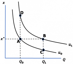
which results in an indifference curve for individual  looking like that depicted in Figure 6.1.

Figure 6.1. Indifference Curve for Envious and/or Guilt-Ridden Homo sapiens

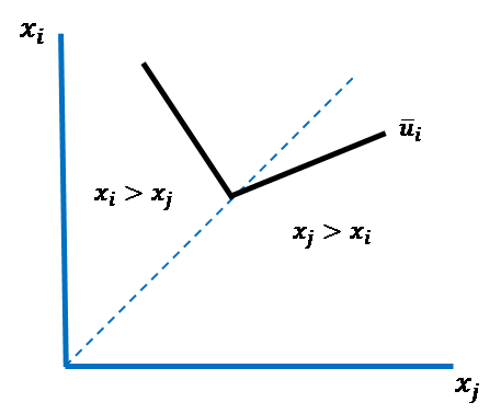
Note that this indifference curve now depicts the interpersonal tradeoff between the two individuals’ wealth levels, and , rather than the intrapersonal tradeoff between the two physical quantities, and , exhibited by individual alone. Recall that when wealth levels are such that , individual is prone to feelings of guilt and is thus confined to the region above the 45° hashed line in the graph. From our formula for the indifference curve above, we see that the slope of the indifference curve’s line segment in this region of the graph is equal to . The value of this fraction in turn measures the (constant) rate at which individual is willing to sacrifice, or transfer, some of her wealth to individual to assuage her guilt at having more wealth (note that any point above the 45° line indicates that individual ’s wealth exceeds individual ’s). The larger is , the more steeply sloped is the line segment, implying that individual feels a greater sense of guilt from her wealth differential with individual , and thus, is willing to transfer even more of her wealth to per unit of ’s wealth.

You might be wondering what the terminology “per unit of ’s wealth” means in this instance. Given that a dollar of wealth to individual  is equal to a dollar of wealth to individual , doesn’t this mean that  must equal 0.5, implying that  (i.e., wealth transfers occur on a one-to-one basis in dollars)? In the present context, the answer is “no.” In cases where , individual  feels so guilty that she would willingly transfer more than $1 of her wealth for each $1 of wealth individual  receives. Talk about feeling guilt-ridden!

In contrast, when wealth levels are such that , and therefore, individual is prone to feelings of envy, individual is confined to the region below the 45° hashed line in Figure 6.1. Again, appealing to our formula for the indifference curve above, we see that the slope of the indifference curve’s line segment in this region of the graph is equal to . The value of this fraction in turn measures the (constant) rate at which individual believes his own wealth should be compensated as individual ’s wealth increases. Note that larger values of indicate larger feelings of envy. However, the upper bound on is equal to 0.5 (rather than 1, as for ) because, as can be seen in the graph, if , then the indifference curve’s associated line segment will automatically cross into the guilt region (where ) and thus, be inconsistent with feelings of envy. In other words, individual ’s wealth cannot be such that she simultaneously feels envy and guilt about individual ’s wealth level.

Fairness in the Context of Framing

Consider the following two experiments conducted by Kahneman (2011):

Confronted with these two experiments, Homo economicus is not fooled by what’s known as “money illusion.” She knows the difference between nominal and real changes and the importance of making decisions based upon the latter. As a result, Homo economicus recognizes that both experiments ask her to rate the fairness of a company’s decision in the face of a recession that is effectively costing the company’s employees (i.e., those employees who have been able to retain their jobs with the company during the recession) 7% of their incomes in real terms. In Experiment 1, this 7% loss in real income results from the company’s decision to reduce wages and salaries by 7% in the face of no price inflation. In Experiment 2 the loss occurs as a result of the company raising wages and salaries by 5% in the face of 12% price inflation. Thus, in separate samples of Homo economicus, we would expect roughly equal percentages of subjects to choose numbers 1 – 5 across the two samples, and for the distribution of percentages to be roughly uniform across the numbers (e.g., 20% choosing 1, 20% choosing 2, etc.).

You probably won’t be too surprised to learn that when Kahneman ran this experiment with his students, 62% chose 4 or 5 in Experiment 1 while only 22% chose 4 or 5 in Experiment 2. Clearly, context matters here for Homo sapiens. In this case, the context broaches the principle of “dual entitlement” in the mind of Homo sapiens, a principle where both the employer and employees are entitled to levels of benefit provided by some “reference transaction.”

The context in Experiment 2 is framed as being less unfair than the context in Experiment 1 simply because the company in Experiment 2 appears to be doing something more to protect its employees’ wages and salaries in the face of inflation than the company in Experiment 1. After all, the company in Experiment 2 is increasing wages and salaries, not lowering them. Unfortunately, the larger percentage of students rating the company in Experiment 1 as being more unfair have been framed. They suffer from money illusion.

Kahneman et al. (1986a; 1986b) ran additional experiments to measure Homo sapiens’ penchant for fairness in other contexts. For example, the authors posed the following experiment to approximately 200 adult residents in the Vancouver metropolitan area of British Columbia, Canada:

Being a devoted practitioner of hard, cold economic efficiency, Homo economicus would rank the auction first, as this would allocate the tickets to the fans willing to pay the most for them, and queueing last, as this is the most economically wasteful way to allocate resources. To Homo economicus, economic efficiency and fairness are one and the same. Unsurprisingly, Kahneman et al.’s participants completely reversed Homo economicus’ ranking. The great majority of the sample ranked queueing as fairest and the auction as the least fair.

In a second set of experiments, the authors contacted adult residents living in the Vancouver and Toronto metropolitan areas and posed the following two experiments to two separate samples of participants:

While we would expect Homo economicus to rate the decisions by both the landlord in Experiment 1 and the shop owner in Experiment 2 as “completely fair,” what about Homo sapiens? Given what we (think we) know about their penchant for fairness, we might expect Homo sapiens to rate both the landlord and shop owner as “very unfair” or at least “somewhat unfair.” Surprisingly, Homo sapiens are not that predictable.

While the great majority of participants rate the shop owner as “somewhat unfair” or “very unfair,” they view the landlord as being “completely fair” or “acceptable.” What’s going on here? Kahneman et al. propound two rules governing the fairness judgments made by participants in the respective experiments. In Experiment 1, it is acceptable for the landlord to maintain her profit level at its reference level by raising rent as necessary, even when doing so causes considerable loss or inconvenience for the tenant. To the contrary, in Experiment 2 it is unfair for the shop owner to exploit an increase in his market power to alter his profit from its reference level at the direct expense of an employee.

As these experiments demonstrate, Homo sapiens consider fairness to be context-specific.

Regret and Blame

Consider the following experiments proposed by Kahneman (2011):

Because Homo economicus ignores possible reference points (i.e., is reference independent) and narrowly frames decisions like this, he is not influenced by Winona’s and Alfred’s past experiences with hitchhikers. Thus, Homo economicus would have no reason to assign greater regret to Winona or Alfred in Experiment 1, or more criticism (i.e., blame) to one or the other in Experiment 2. When it comes to assigning greater regret and more blame, Homo economicus essentially flips two fair coins—if “heads” then assign greater regret and more blame to Winona, “tails” assign them to Alfred. We would consequently expect respective samples of Homo economicus to assign greater regret and more blame 50%-50% to Winona and Alfred.

Kahneman’s experiments with his students resulted in 88% assigning greater regret to Winona, and 77% assigning more blame to Alfred. Therefore, appears that Homo sapiens are prone to using a social norm as their reference point when deciding how to apportion regret and blame to people like Winona and Alfred. In this case, the norm is “do not pick up hitchhikers.” The logic for how this norm cum reference point could be driving Homo sapiens’ choices in these experiments goes something like this:

Because Alfred has frequently (and presumably knowingly) flaunted this norm in the past, “he had it coming to him,” and thus, “should have seen it coming.” Alfred is, therefore, not entitled to feel as much regret as does Winona, who, by contrast, has rarely if ever flaunted the norm. Winona was less likely to see the robbery coming and likely feels greater regret at having transgressed a norm that she has traditionally followed. Because Alfred has traditionally transgressed the norm and had the robbery coming to him, he effectively deserves to be more severely criticized.

Hopefully, you see that, as compelling as this logic seems, it is misguided. With respect to regret, the question pertains to what we think Winona and Alfred will feel about themselves after having been robbed (think Regret Theory from Chapter 4), not what we think they are entitled to feel. Similarly, regarding the apportionment of blame, we know nothing about the people who will be judging the two victims, in particular, how they tend to judge others’ behaviors. In the end, then, this is a case where narrowly framing the situations and avoiding the use of reference points would actually help Homo sapiens reach more judicious judgments.

Asymmetric Regret

Consider the following thought experiment conducted by Kahneman (2011):

Similar to how she interpreted the human emotion of regret in the previous experiment, Homo economicus will again ignore potential reference points and narrowly frame her judgment (i.e., she will not abide by the strictures of Regret Theory). In the final analysis, Cheryl and Wilbur both lost $25,000 by choosing to hold stock in Company A. It doesn’t matter that Cheryl held onto the stock rather than switching to stock in Company B, or that Wilbur switched from owning stock in Company B to owning stock in Company A. They both lost $25,000, and should therefore both feel the same amount of regret.

Not so with Homo sapiens. Kahneman reports that 92% of his subjects assigned a greater sense of regret to Wilbur than to Cheryl. The reference point here pertains to whether an investor decides to switch ownership in a stock or not. The logic goes something like this:

When the value of their stock in a given company falls, investors who exhibit inertia and choose not to sell their ownership in that stock beforehand later experience less regret than investors who instead choose to purchase ownership in that stock beforehand. In this case, the proverb “fools rush in where angels fear to tread” implies that when what the fools rushed into costs them money, they should feel more regret than the angels who lost the same amount of money by instead exhibiting more patience.

Yeah, right. Their propensity for broad framing and reference-dependent decision-making has apparently again led Homo sapiens astray (“apparently” being an important word here). Perhaps Kahneman’s subjects should have instead flipped fair coins and tried not to reason their ways to answers. Or not. Could there be a more compelling logic for Kahneman’s results?

One could argue that, to the extent Kahneman’s subjects believed Cheryl and Wilbur are prone to what we previously learned in Chapter 4 is called the Endowment Effect, then the subjects were justified in concluding that Wilbur suffers more regret than Winona. An Endowment Effect occurs when the intrinsic value associated with owning something (e.g., a given commodity) is large enough to induce the owner to unwittingly overprice the commodity in a market setting.^[9] Therefore, if Wilbur is susceptible to the Endowment Effect—specifically a retroactive Endowment Effect associated with the shares he once owned in Company B—then it is very likely he is suffering more regret than Winona by having forfeited that endowment. Because she never actually owned stock in Company B, Winona is perforce precluded from the opportunity to suffer an Endowment Effect.

It is important to note that this is not a case of “two wrongs making a right.” While it may be “wrong” for Wilbur to exhibit an Endowment Effect, it is not wrong for Kahneman’s subjects to assume that he does. Indeed, one could argue that to the extent Kahneman’s subjects made this assumption, they made the correct choice—correct not just because they honored the assumption but also because (as will be discussed in Section 3) Homo sapiens really are prone to this effect.

Once a participant submits an answer on the computer, a new problem appears jointly with information on whether the former answer was correct. This process continues for five minutes. A record of the participant’s number of correct and wrong answers remains on the screen as s/he progresses through the five-minute set of problems. Their final scores are determined by the number of correctly solved problems in the five-minute timespan. Niederle and Vesterlund (2007) chose this approach because it requires both skill and effort and because there was no prior evidence in the extant literature of gender differences in ability on easy math tests. The authors were, therefore, able to rule out performance differences as an explanation for gender differences in the choice of competition level (i.e., choice between the noncompetitive piece-rate and competitive tournament schemes).

Participants were randomly divided into groups of four, each group seated in a row. Participants were informed that they were grouped with the other people in their row. Each group consisted of two women and two men. Although gender was not discussed at any time, participants could see who the other people in their group were and were thus aware of their group’s gender mix. A total of twenty groups participated in the experiment (40 men and 40 women total). Each participant received a $5 “show-up fee” and an additional $7 for successfully completing the experiment.

Participants were instructed to complete four separate sets of math problems (i.e., four separate tasks) and were told that one of these tasks would be randomly chosen for payment after the experiment. While each participant could track their own performance on any given task as the math problems were completed, they were not informed of their relative performance to everyone else in their group until the end of the experiment (i.e., upon conclusion of the fourth task). Under the piece-rate scheme, participants earned $0.50 per correct answer. Under the tournament scheme, the participant who correctly solved the largest number of problems in the group received $2 per correct answer while the other participants received no payment. In case of ties, the winners were chosen randomly from among the high scorers.

Task 1 was presented to each participant under the piece-rate scheme, and Task 2 was presented under the tournament scheme. These initial tasks were meant to serve as baseline measures of each participant’s performance under the two schemes. Under Task 3, participants selected whether they wanted to be paid according to the piece-rate or the tournament scheme before engaging in the task. A participant choosing the tournament received $2 per correct answer if her score in Task 3 exceeded that of the other group members in Task 2’s tournament they had previously completed. Otherwise, he received no payment. Again, in case of ties, the winners were chosen randomly. Thus, participants choosing to play in a tournament in Task 3 are competing against other participants who had already participated in the two previous tasks, which enabled Niederle and Vesterlund to rule out the possibility that women might shy away from competition because by winning the tournament they would impose a negative externality on the other group members.

Lastly, under Task 4, the participants were not presented with a new set of math problems. Rather, if this task was randomly selected for payment at the end of the experiment, a participant’s compensation would depend upon the number of correct answers s/he provided under Task 1’s scheme. In Task 4, a participant could choose which compensation scheme s/he wanted applied to his or her past performance in Task 1, piece rate or tournament. A participant would therefore effectively win a Task 4 tournament if his or her Task 1 performance had been the highest among the other participants in the group for that task. Before making their choices in Task 4, participants were reminded of their respective Task 1 performances. Thus, Task 4 allowed Niederle and Vesterlund to see whether gender differences in the choice of compensation scheme appeared even when no future and past tournament performance was involved. The authors could determine whether general factors such as overconfidence, risk, and feedback aversion caused a gender gap in the choice between the noncompetitive piece-rate and competitive tournament schemes. At the end of the experiment, before learning about their performance relative to the group’s other participants, each participant was asked to guess her ranking (in terms of the number of correctly solved problems) in Tasks 1 and 2, respectively. Each participant picked a rank between 1 and 4 and was paid $1 for each correct guess.

As expected, the authors found no statistically significant gender gap in performance under either the piece-rate or tournament schemes, with both sexes performing significantly better in a tournament. As a result, Niederle and Vesterlund conclude that there is no gender difference in the probability of winning the Task 2 tournament. More importantly for this particular experiment, the absence of a gender gap in the performance of Tasks 1 and 2 raises the expectation that a subsequent gender gap in Task 3 should likewise not be observed. However, this expectation was not fulfilled—35% of women and 73% of men selected the tournament, a statistically significant result. Moreover, as the figure below demonstrates, at each Task 2 performance level, men are more likely to enter the tournament in Task 3 (the figure’s vertical axis measures the percentage of the group entering the tournament). Even women who score in the highest (“best”) performance quartile chose to enter the tournament at a lower percentage than men in the lowest (“worst”) performance quartile.

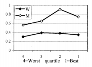
In other words, while women shy away from competition, men are drawn to it.

Turning to Task 4, recall that although this choice is very similar to that of Task 3, Task 4’s choice eliminates the prospect of having to subsequently participate in a competition. Thus, only in Task 3 could a gender gap in preference for competition have played a role in the choice of compensation scheme. As the figure below shows, there is no statistically significant gender gap in the choice of compensation scheme in Task 4 based upon perceived ranking in Task 1. A higher percentage of women than men who guessed their Task 1 ranking to be low (i.e., at level “3”) chose the tournament scheme in Task 4, while the percentages were reversed for those participants who guessed their Task 1 rankings to be high (at levels “1” and “2”). But because the two lines in the figure remain close together, these differences are not statistically significant (i.e., we should treat the groups’ respective choices as being no different from one another).

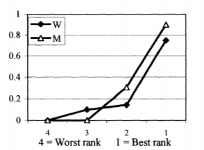
This result from Task 4 cements the authors’ finding that women shy away from actual competition slated to occur at a future point in time, not implicit competition based upon their interpretations of how their past performance compares with others.^[10]

Testing for the Existence of an Endowment Effect

Here is an experiment you and your fellow students can use to test the extent to which you exhibit an Endowment Effect—an experiment facilitated by your instructor, of course:^[11]

For example, suppose from a class with 10 students, we randomly select five to be sellers and five to be buyers of the coffee cup. Each buyer and seller writes his or her price on a sheet of paper, and the outcome is tallied.

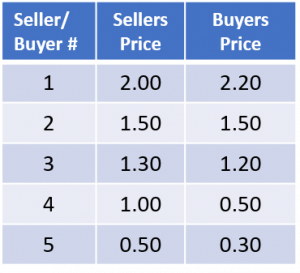
In this “market,” an equilibrium occurs where Buyer 1 pays Seller 1 $2.00 for Seller 1’s cup, Buyer 2 pays Seller 2 $1.50 for Seller 2’s cup, Buyer 3 pays Seller 4 $1.00 for Seller 4’s cup, and Buyer 4 pays Seller 5 $0.50 for Seller 5’s cup. Seller 3 does not end up selling and Buyer 5 does not end up purchasing a coffee cup. To see this, first note that Buyer 1’s offer price (or willingness to pay (WTP)) exceeds Seller 1’s asking price (or willingness to accept (WTA)), which is the largest WTA value among the group of sellers. Thus, Buyer 1 and Seller 1 are “matched,” and Seller 1 is paid his WTA. Next, since Buyer 2’s WTP just matches Seller 2’s WTA (which is the next highest WTA value), Buyer 2 and Seller 2 are matched. The next highest WTP value is exhibited by Buyer 3, and since this value exceeds Seller 4’s WTA (not Seller 3’s), Buyer 3 is matched with Seller 4. Finally, Buyer 4’s WTP just matches Seller 5’s WTA, so Buyer 4 and Seller 5 are matched. In the end, no such matches can be found for Buyer 5 and Seller 3.

This is good information to have. But a question remains: is there evidence of an Endowment Effect in this market?

The answer is (most likely) “no” since four out of five possible sales were ultimately consummated. Although there is no hard-and-fast threshold for determining whether the effect has occurred, it seems safe to say that wherever one might put the threshold, four-out-of-five (or 80% of possible sales consummated) would lie above it. Or, to put it another way, in a market characterized by a relatively strong Endowment Effect exhibited by its sellers, one would expect most sellers’ WTA values to exceed buyers’ WTP values, resulting in few sales ultimately being made. Indeed, if pressed to nail down a threshold, one can really do no better than to metaphorically flip a coin (i.e., to choose a 50% threshold), which, in the case of our example market, means that only one or two consummated sales would have indicated the existence of an Endowment Effect.

Homo economicus and the Endowment Effect**

In Chapter 3 we introduced the graphical concept of an indifference curve. We mentioned that the stylized version of this curve—smooth, everywhere downward-sloping, and convex to the origin—can be used to represent Homo economicus’ preferences over any two commodities. It turns out that this framework, as demonstrated in Hanley et al. (2007), can be used to reach an interesting conclusion about Homo economicus’ susceptibility to the Endowment Effect.

In Figure 6.2 below, two indifference curves are drawn for our individual whom we’ll name Ted, each curve corresponding to a different level of utility, and . Recall that the relative locations of the two curves indicate that (i.e., the curve drawn for utility level corresponds to a set of bundles yielding a higher level of utility than the set of bundles denoted by the curve drawn for ).^[12]

Figure 6.2. Homo economicus and the Endowment Effect

For sake of example (but without loss of generality), Ted’s two indifference curves have been drawn for two commodities denoted as and . Commodity is a “private good” that Ted has to purchase directly with his income. Commodity is a “public good” that Ted receives from the government without having to make a direct payment out of his income (e.g., more wilderness area for Ted to explore near his home, cleaner air for Ted to breath, etc.). We assume that commodities and are the only two commodities Ted consumes.^[13] Also identified in Figure 6.2 are points A – D, level for commodity , and levels and for commodity . Finally, for future reference we note that because Ted can only spend his income on commodity , he ends up spending all of his income on, which means he’s stuck with consuming level regardless of whether he consumes level or of commodity Q. Therefore, the higher is located on the vertical axis, the larger is Ted’s income level, all else equal.

Okay. We are now ready to show why Ted, our Homo economicus, exhibits an Endowment Effect. We start by assuming that Ted initially consumes at point A (i.e., bundle ) where he attains utility level . Now, let the level of the public good increase from  to . Note that because Ted is constrained to consume level  of commodity , we know that he now consumes at point B where he attains the higher level of utility . It makes sense that Ted is happier at point B because he is now consuming the same amount of commodity  at that he was originally consuming at point A, and he also gets to consume more of commodity  (lucky him).

It turns out that vertical distance AC in Figure 6.2 represents Ted’s WTP for this move from point A to point B. How so? Distance AC represents the maximum amount of commodity that we could take away from Ted such that (1) his consumption of commodity is maintained at level , and (2) Ted is not left with fewer utils than his initial utility level, . Hence, vertical distance AC indeed represents Ted’s WTP for the change in the level of good represented by (measured in terms of commodity ).

To identify his WTA, we instead start by assuming that Ted initially consumes at point B (i.e., bundle ) where he has attained utility level . Now, let the level of the public good decrease from to (i.e., some of the public good has been taken away from Ted—the wilderness area near his home has shrunk, or air quality has worsened, etc.). Note that because Ted is again constrained to consume level of commodity (because his income level has remained the same), we know that he now chooses to consume at point A where he regresses to the lower level of utility . It makes sense that Ted is less happy at point A because he is now consuming the same amount of commodity at A that he was originally consuming at B and is, unfortunately, consuming less of commodity (woe to him).

Adopting a similar logic, vertical distance AD in Figure 6.2 represents Ted’s WTA for this move from point B to point A. In this case, distance AD represents the minimum amount of commodity we must give Ted such that this amount (1) holds his consumption of commodity at level and (2) does not leave Ted with less than his initial utility level, . Hence, vertical distance AD indeed represents Ted’s WTA for the change in the level of good represented by (again, measured in terms of commodity ).

Recall that WTP and WTA both measure Ted’s valuation of a given change in the amount of public good . However, the contexts within which the measurements occur are different. WTP presumes Ted does not initially own rights to the change in the amount of the good—it is his maximum willingness to pay to gain ownership of that changed amount. In contrast, WTA does presume that Ted initially owns rights to the change in the amount of the good—it is his minimum willingness to accept the loss of ownership of that changed amount. Thus, if Ted’s WTA exceeds his WTP for the same amount of change in good , then he exhibits an Endowment Effect. This is because he would then place a higher value on amount relative to when he initially owns as opposed to when he does not. In other words, Ted places a higher value on the change in the amount of simply because he is endowed with the right to own that changed amount. Clearly, distance AD exceeds distance AC in Figure 6.2, implying Ted’s WTA is greater than his WTP for the given change in the amount of good . Thus, even a Homo economicus like Ted exhibits an Endowment Effect.^[14]

Concluding Remarks

Recall that the goal of Section 2 is to explore exactly where the standard, rational-choice theory ascribed to Homo economicus fails to adequately predict behavior we repeatedly see exhibited by Homo sapiens in laboratory and field experiments. We have learned that, in several key respects, this behavior systematically violates the theory. The violations appear in a myriad of forms; as violations of axioms known as Dominance, Invariance, Independence, and Substitution, and the Sure-Thing Principle. From these violations spring two questions—why and toward what ends? The question “why” pulls us back into the realms of cognitive and psychological sciences, realms rich in reminders of what makes Homo sapiens so exquisitely quirky and idiosyncratic and inherently fallible. And the question “toward what ends” propels us forward into the realm of understanding where and how rational-choice theory fails to adequately explain human choice behavior. In this realm, the new theories of behavioral economics arise.

Following Kahneman (2011) and others, we call these quirks and idiosyncrasies, “miscalculations, biases, fallacies, heuristics, and effects.” We recall specific terminology such as Affect and Availability Heuristics, Priming and Framing Effects, Status Quo and Confirmation Biases, Conjunction Fallacy, the Law of Small Numbers, conformity, mental accounting, and the overweighting of improbable events, among others. These are the types of human foibles distinguishing Homo sapiens from Homo economicus. They materialize as violations of rational choice theory. As we have learned, the violations were identified in the foundational laboratory experiments conducted by Nobel Laureates Daniel Kahneman and Richard Thaler, among many others, experiments that you and your classmates have now participated in yourselves.

It is one thing to identify where a body of theory fails to adequately explain real-world phenomena. It is another to revise that theory in an effort to advance not only the theory but also to gain a deeper understanding of the human experience itself. Toward this end, we have learned about the value function and how it can be used to depict such behaviors among Homo sapiens as reference dependence, loss aversion, and the Endowment Effect. And we have learned about the complications imposed on the rational-choice theory by human emotions such as envy, guilt, regret, and blame, as well as Homo sapiens’ discomfiture with ambiguous circumstances and the need to feel and appear competent.

Study Questions

Note: Questions marked with a “†” are adopted from Just (2013).

1. ^† Which of the two utility functions represents transactional utility and why?   and  , where  represents the total amount of a good purchased, and  represents the total cost incurred by the consumer in purchasing the good.
2. Why might people be more likely to spend a small inheritance and invest a large one? Which quirk of Homo sapiens introduced in this chapter does this likelihood represent?
3. ^† How does the use of a credit card confound the conclusion reached by Prelec and Loewenstein (1998); namely that, as an example of mental accounting, Homo sapiens seem to prefer decoupling payments for durable goods but not necessarily for non-durable (perishable) goods?
4. Can you think of an example from your own life where you have practiced mental accounting? Explain.
5. ^† Ella is a high school student who is given $3 each school day by her parents to be used as “lunch money.” She works a part-time job after school, earning a small amount of “spending cash.” In addition to her lunch money, Ella spends $5 from her spending cash each week on lunch. Suppose her parents reduced Ella’s lunch money by $2 per day but that she simultaneously receives a $10-per-week raise at her job, requiring no extra effort on her part. What would the rational choice model suggest should happen to Ella’s spending on lunch? Alternatively, what does the mental accounting framework predict?
6. Each year, hundreds of thousands of people receive coronary-artery bypass surgery. The surgery saves their lives, but only for the long term if they adopt some important lifestyle changes such as dietary changes, quitting smoking, more physical exercise, and managing stress more effectively. Suppose Hayden the Hyperbolic Discounter, who has a hankering for eating junk food, smokes cigarettes occasionally when stressed out, and avoids regular exercise, decides to have coronary bypass surgery. What do you think the long-run outcome is going to be for Hayden?
7. Which experiment discussed in this chapter do these results pertain to?
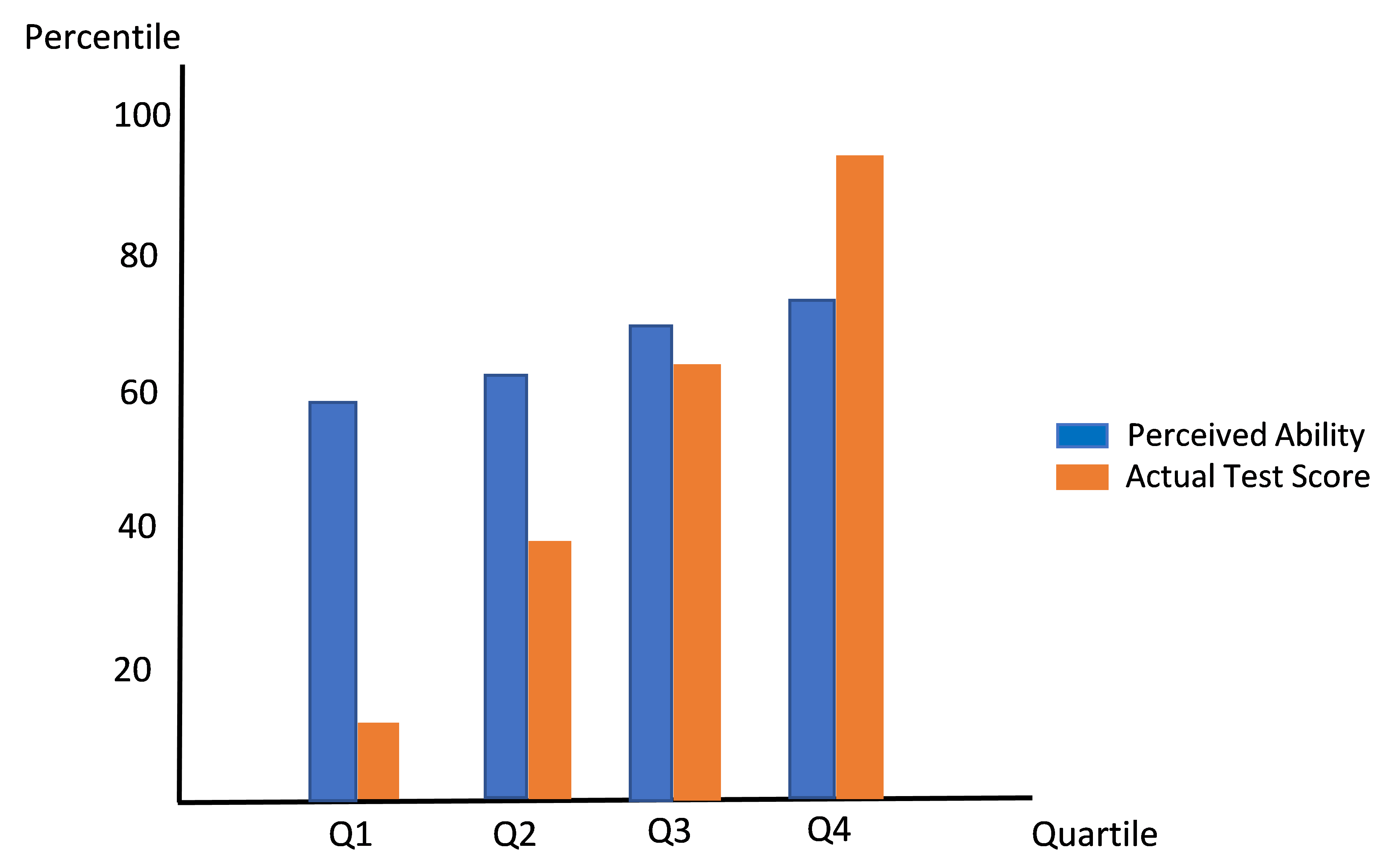
8. Suppose Evelyn the Environmental Economist is presenting her case in a public meeting for why raising the price of municipal water in the face of persistent drought conditions would be a good thing for the community, when someone in the audience yells out, “That’s unfair for seniors and others living on fixed incomes.” How might Evelyn frame her response in a way that dispels the audience’s concerns about the fairness of a price increase?
9. How would the indifference curve in Figure 6.1 change when drawn for a person who suffers from guilt but not envy? Draw the curve.
10. Can you recall an example from your own life where you exhibited an Endowment Effect that ultimately led to regret?
11. The Gender Gap experiment discussed in this chapter measured gender differences in terms of how males and females deal with competitive situations. Think of another situation where a gender gap may exist and design an experiment to test for it.
12. It was shown in this chapter that a Homo economicus who exhibits convex-shaped indifference curves exhibits an Endowment Effect. Does this result still hold if Homo economicus exhibits linearly shaped indifference curves, as depicted in the figure below? Show your result using this graph.
    
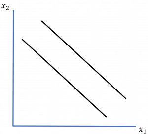
13. Explain the relationship between the Decoy Effect and reference dependence. Describe a situation in your own life where you have been a victim of the Decoy Effect.
14. Describe a negative implication of the Zero-Price Effect in the real world. Have you ever fallen victim to this effect in your own life? If so, describe the circumstances.