8 Some Classic Simultaneous-Move Games
Prisoner’s Dilemma
This is undoubtedly one of the most well-known simultaneous games Homo sapiens play (for the most part unwittingly) in their day-to-day lives. Prisoner’s Dilemmas abound in our social interactions, in particular, governing how we manage natural resources collectively. You may have heard of the “tragedy of the commons” when it comes to managing fisheries, rangelands, local watersheds and airsheds, or global climate change. It turns out that a Prisoner’s Dilemma is at the root of these types of resource management challenges. It is a dilemma that confronts us daily and drives individual decision-making in a social setting.
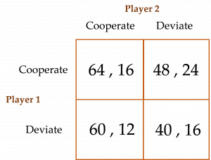
The game is presented below in its “strategic form”—a matrix containing the payoffs each of the two players will obtain from their respective choices when they move simultaneously as opposed to sequentially.[1] There is common knowledge in this game in the sense that Player 1 knows not only her payoffs listed in the matrix, but also Player 2’s. Player 2 likewise knows not only his payoffs, but also Player 1’s. The payoff matrix for a Prisoner’s Dilemma game is depicted below:
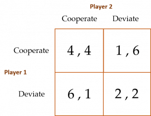
In this game, both players simultaneously choose whether to Cooperate or Deviate. If both players choose Cooperate, then they both receive payoffs of $4 each. If both instead choose Deviate, then they receive payoffs of only $2 each. If Player 1 chooses Cooperate but Player 2 chooses Deviate, then Player 1 receives a payoff of only $1 while Player 2’s payoff jumps to $6. Likewise, if Player 1 chooses Deviate when Player 2 chooses Cooperate, then Player 1’s payoff jumps to $6 and Player 2’s falls to $1.
Because moves in this game are made simultaneously, the solution concept is not SPE or BPE. Rather, it is either a “pure strategy equilibrium” or a “mixed strategy equilibrium.” It turns out that the Prisoner’s Dilemma solves for a unique pure strategy equilibrium (PSE). We will encounter simultaneous games that solve for mixed strategy equilibria (MSE) a bit later in this chapter.
The logic for this game’s analytical PSE goes like this:
Both players consider their payoffs associated with Cooperate or Deviate given what the other player could decide to do and, in this way, devise their respective strategies. For instance, Player 1 first considers her payoffs when Player 2 chooses to Cooperate. Because $6 > $4, Player 1’s best strategy is to Deviate when Player 2 chooses to Cooperate. Next, Player 1 considers her payoffs when Player 2 chooses to Deviate. Because $2 > $1, Player 1’s best strategy is again to Deviate when Player 2 chooses to Deviate. Because Player 1’s best strategy is to Deviate regardless of whether Player 2 chooses to Cooperate or Deviate, we say that Player 1 has a “dominant strategy” to choose Deviate no matter what Player 2 decides to do! Applying the same logic to Player 2’s decision process, we see that Player 2 also has a dominant strategy to choose Deviate no matter what Player 1 decides to do. Thus, the PSE for this game is both players choosing to Deviate (i.e., (Deviate, Deviate)).[2]
What a shame! Both players choose to Deviate, and, as a result, they attain payoffs of only $2 each. This equilibrium is woefully inefficient. Had the two Homo economicus not been so self-interested and oh so rational, perhaps they could have agreed to Cooperate and earned $4 each instead of just $2. Such is the essence (and bane) of the Prisoner’s Dilemma.[2]
Ironically (or should I say, sadly), when Homo sapiens play this game, they tend to attain the analytical PSE, although cooperation has been found to occur in some experiments (c.f., Heurer and Orland, 2019). This should come as no surprise. As we now know, the Prisoner’s Dilemma (and Homo sapiens proclivity for attaining the game’s PSE) is a contributing factor to historically intractable resource management problems in everyday life like air pollution, water scarcity, and climate change.[3]
Finitely Repeated Prisoner’s Dilemma
Similar to the question of whether repeatedly playing the trust game for multiple stages could lead to greater trust and trustworthiness among an Investor and Trustee, the question arises as to whether repeated play of the Prisoner’s Dilemma can lead to more cooperation among two players in a PSE. Unfortunately, applying backward induction to the payoff matrix above for a finite number of periods suggests that the answer is “no.” To see this, suppose two players are in the final stage of the game. Given the payoff matrix above, (Deviate, Deviate) is the PSE. Knowing this, in the penultimate stage, both players have no better options than to choose (Deviate, Deviate) again. Similar to the centipede game where mutual mistrust unfolds all the way back to the initial round, here, mutual deviation unfolds back to the first stage. Analytically speaking, cooperation does not emerge in a finitely repeated Prisoner’s Dilemma game—repeatedly deviating is the dominant strategy for both players.
Nevertheless, Kreps et al. (1982) and Andreoni and Miller (1993), among others, find that Homo sapiens tend to cooperate more when they are uncertain of the other player’s tendency to cooperate. Furthermore, Spaniel (2011) demonstrates that when players adopt strategies such as “grim trigger” and “tit-for-tat” in an infinitely repeated Prisoner’s Dilemma game, cooperation is more likely to occur. Grim trigger is a strategy where if your opponent Deviates at any stage, you Deviate forever starting in the next stage. Otherwise, you continuously Cooperate. Tit-for-tat is where you begin by choosing to Cooperate. In future stages, you then copy your opponent’s play from the previous period.[4]
Public Good Game
As in the Prisoner’s Dilemma, the dominant strategy in a Public Good Game results in a PSE among Homo economicus, and often among Homo sapiens, that is inefficient when compared with what would otherwise be a cooperative outcome. In a simple version of this game—called a linear public good game—there is a group of  players, each of whom receives an initial allocation of money, say $10, and then is asked how much of that $10 she will voluntarily contribute to a group project of some kind. Each dollar that is donated by an individual player to the group project is multiplied by some factor
  ,
,  , and shared equally among all members of the group (for the sake of a game played in a laboratory, the group project is simply a pot of money). The fact that ensures that an individual player’s contribution to the pot of money is larger in value for the group as a whole than it is for that individual.
For example, suppose there are four players (including you) and = 2. If you contribute a dollar to the pot, then you give a dollar and receive only $0.50 out of the pot in return (($1 x 2) ÷ 4 players = $0.50). However, for every dollar contributed by another player, you receive $0.50 out of the pot, free and clear. You can see how this game mimics the social dilemma Homo sapiens face when it comes to voluntarily financing a myriad of public goods (or group projects) such as public radio and public TV, environmental groups, and political campaigns, to name but a few. Each dollar contributed by someone else gives you additional benefit associated with a larger public good, for free. You get that same additional benefit from the public good when you are the one contributing but at the cost of your contribution.
Since the overall return the group gets from your dollar contribution exceeds the dollar (recall that in our case the overall return is $1 x 2 = $2 per dollar contributed), it is best (i.e., socially efficient) for each group member to contribute their full $10 allocation. The socially efficient equilibrium to this game earns each player a total of $20 (($10 x 2 x 4 players) ÷ 4 players = $20). In contrast, because each player only gets back $0.50 for each dollar contributed, there is no individual incentive for a player to donate any amount of money (or, to put it in economists’ terms, there is a strong incentive for each player to “free ride” on the generosity of the other players’ contributions). Thus, the PSE for this game—again, the equilibrium we expect Homo economicus players to obtain as a consequence of their self-interested, rational mindset—is where each player free rides and contributes nothing. Grim, but true.
One way to convince yourself that the PSE for the Public Good Game is where each player contributes zero to the group project is to start at some arbitrary non-zero contribution level for each player and then show that each player has an incentive to reduce their contribution to zero. For example, suppose the starting point in our game is where each player contributes $6 to the money pot. This means that each player would receive a total of $12 from the pot (($6 x 2 x 4 players) ÷ 4 players =$12). Thus, each player takes home from the game a total of $12 + $4 = $16. Now suppose one of the players decides instead to free-ride by dropping her contribution to $5. Each of the four players now receives $11.50 from the money pot ([($6 x 2 x 3 players) + ($5 x 2 x 1 player)] ÷ 4 players = $11.50). The total take-home pay for the three non-free-riding players is now $11.50 + $4 = $15.50, while the free-riding player takes home $11.50 + $5 = $16.50. Clearly, the free-riding player is better off by having dropped his contribution to $5, and the three non-free-riding players are each worse off. But then each of the non-free-riders would recognize that they too would have been better off by free-riding, just like the free-rider. So, they too have equal incentive to free-ride. Barring any type of pre-commitment made by each of the players, this free-riding process cascades to each player choosing to fully free-ride or, to use the Prisoner’s Dilemma lingo, to “deviate” from what is otherwise a fully cooperative equilibrium where each player contributes their total $10 to the money pot. Voila, we arrive at a PSE where each player chooses to contribute zero to the money pot.
Taking their cue from the likes of Kreps et al. (1982) and Andreoni and Miller (1993) in testing a finitely repeated version of the Prisoner’s Dilemma Game, Fehr and Gächter (2000) explore whether a finitely repeated Public Good Game likewise mitigates deviation on the part of the players (i.e., free-riding behavior). The authors construct four treatment groups of student subjects. There is a “stranger treatment,” with and without punishment opportunities, and a “partner treatment,” with and without punishment (punishment in this context is explained below). In the partner treatment, 10 groups of four subjects each play the linear public good game for ten rounds without punishment and ten rounds with punishment, with group composition remaining unchanged across rounds (hence, the title, “partner treatment”). In contrast, in the stranger treatment, a total of 24 subjects are randomly partitioned into groups of four players in each of the twenty rounds (10 rounds without punishment and 10 rounds with punishment). Group composition in the stranger treatment changes randomly from round to round. In both treatments, subjects anonymously interact with each other.
Games played without punishment opportunities serve as a control for games played with punishment opportunities. In a game with punishment opportunities, each subject is provided the opportunity to punish any other player (after any given round) after being informed about each player’s contribution during that round. Punishment in this game takes the form of one player (the punisher) assigning “punishment points” to another player (the punished). For each punishment point assigned to a player, the player’s payoff from that round is reduced by 10% (not to exceed 100%). To mitigate the potential misuse of the punishment mechanism, punishers face an increasing cost associated with assigning punishment points. The cost rises one-for-one with the first two points assigned, and then rises at an increasing rate for points assigned beyond two. Egads, this is sounding a bit complicated.
Fehr and Gächter’s results are depicted in the following two figures: the first figure shows results for groups in the stranger treatment where the first 10 rounds are played without punishment, and the second 10 rounds are played with punishment. The expectation is that the availability of punishment opportunities would lead to an increase in the average player’s contribution to the money pot. This is depicted in the first figure both by the discrete jump in contribution level starting in round 11, and the steady increase in this level over the remaining 10 rounds of the game. The downward trend in contribution levels over the first 10 rounds played indicates that the players learned that cooperation does not pay in a public good game without some form of punishment.
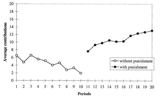
The second figure shows similar results for the partner-treatment groups. What is notable in comparison with the results for the stranger-treatment groups is that (1) the downward trend in the initial 10 rounds becomes noticeably steeper from round seven onward, and (2) the initial jump up in average contribution level starting in round 11 (when punishment opportunities become available) is markedly larger, leading to higher per-round average contributions levels thereafter. These results demonstrate what is commonly known as “reputational effects” associated with a player’s history of contributions over time. Among partner-treatment groups, reputational effects are enabled, while among stranger-treatment groups, they are not.
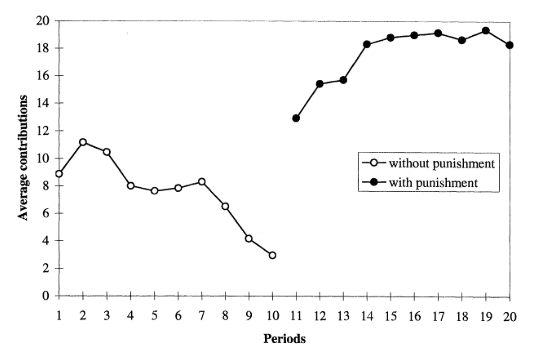
It appears that punishment works with Homo sapiens in repeated play of a Public Goods Game, similar to how punishment works with Homo sapiens in repeated play of a Prisoner’s Dilemma Game.[5]
In addition to enabling punishment opportunities as a “coordinating mechanism” to reverse the grim, inefficient, free-riding equilibrium among Homo sapiens in a finitely repeated Public Good Game without punishment, Rondeau et al. (1999) and Rose et al. (2002) propose a promising mechanism for one-shot games, called the Provision-Point Mechanism. As Rose et al. explain, a provision point mechanism solicits contributions for a public good by specifying a provision point, or threshold, and a money-back guarantee if total contributions do not meet the threshold. Extended benefits are provided when total contributions exceed the threshold. The authors report that the provision point mechanism has led to increased contribution levels (and thus adequate funding for public goods) in their laboratory and field experiments.[6]
Stag Hunt
As its name suggests, this game tests the extent to which hunters can coordinate their efforts to bring down big game. Skyrms (2004) explains the game’s onomatology—the Stag Hunt is a coordination game in which two hunters go out on a hunt together. Each can individually choose to hunt a stag or a rabbit. If one of the hunters hunts a stag, she must have the cooperation of the other hunter to succeed. Thus, like in the Prisoner’s Dilemma, choosing to cooperate is risky—the other hunter can indicate he wants to cooperate but, in the end, take the less risky choice and go after a rabbit instead (remember, like in the Prisoner’s Dilemma, the players’ decisions are made simultaneously in this game). Alone, a hunter can successfully catch a rabbit, but a rabbit is worth less than a stag. We see why this game can be taken as a useful analogy for social cooperation, such as international agreements on climate change. An individual alone may wish to cooperate (e.g., reduce his environmental “footprint”), but he deems the risk that no one else will choose to cooperate as being too high to justify the change in behavior that his cooperation entails.
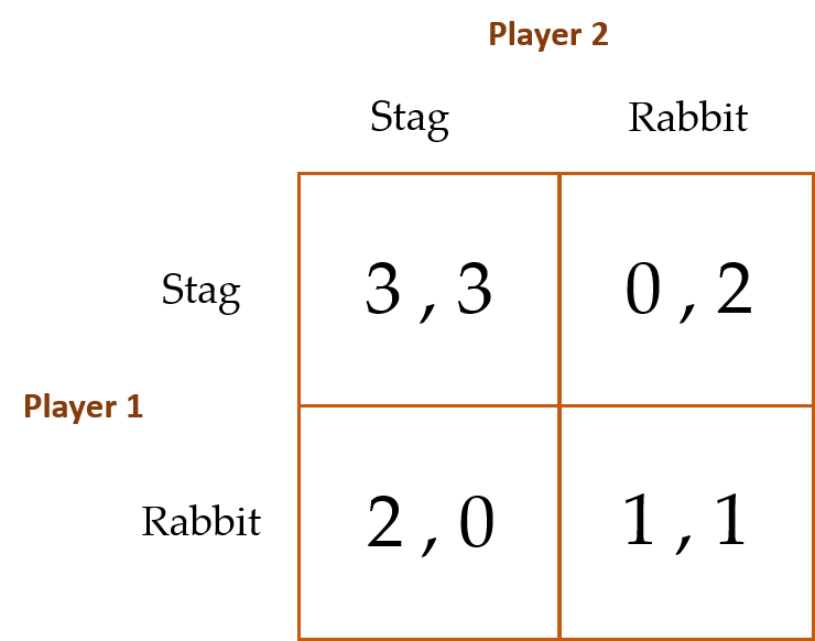
Here is the game’s payoff matrix:
We use the same logic to determine this game’s analytical PSE as we did to determine the Prisoner’s Dilemma:
Player 1 first decides what to do if Player 2 chooses to hunt stag. Because Player 1’s payoff in this case from hunting stag ($3) exceeds his payoff from hunting rabbit ($2), Player 1 will choose to hunt stag when Player 2 hunts stag. Next, we see that when Player 2 chooses to hunt rabbit, Player 1 will also choose to hunt rabbit since, in this case, the payoff from hunting rabbit ($1) exceeds the payoff from hunting stag ($0). Using the same approach to determine what Player 2’s best strategy is, we see that she will also choose to hunt stag when Player 1 hunts stag and will hunt rabbit when Player 1 hunts rabbit. Hence, neither player has a dominant strategy in this game, and as a consequence, there are actually two PSEs. One PSE is where both players hunt stag; the other is where both hunt rabbit. We cannot say for sure which of the two equilibria will be obtained.
Clearly, the (stag, stag) equilibrium is preferable (also known as “Pareto dominant”).[7] But this equilibrium requires that credible assurances be made by each player. In contrast, the (rabbit, rabbit) equilibrium is “risk dominant” in the sense that by choosing to hunt rabbit both players avoid the risk of having gone for stag alone. We would expect this equilibrium to occur when neither player is capable of making a credible assurance to hunt stag. Also note that even though this game does not permit the use of backward induction by the players (as a result of the game consisting of simultaneous rather than sequential moves), each player inherently uses “forward induction” in predicting what the other player will choose to do.
Belloc et al. (2019) recently conducted an experiment where a random sample of individuals playing a series of Stag Hunt games are forced to make their choices about whether to hunt stag or rabbit under time constraints, while another sample of players has no time limits to decide. The authors find that individuals under time pressure are more likely to play stag than individuals not under a time constraint. Specifically, when under time constraints, approximately 63% of players choose to hunt stag as opposed to 52% when no time limits are imposed.
Zero-Sum Game
Consider the following payoff matrix (where, as with the Prisoner’s Dilemma and the Stag Hunt, each player’s payoffs are common knowledge):
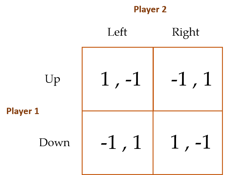
The reason why this matrix depicts a zero-sum game is because the payoffs to Players 1 and 2 sum to zero in each cell. Any time a player wins $1, the other player loses $1. You may have heard someone say, “my gain is your loss” or the other way around, or perhaps you’ve said something like this to someone yourself. When this happens, the two individuals are (unwittingly or not) acknowledging that they are participating in a zero-sum game.[8]
Using the same logic as we used in the Prisoner’s Dilemma and Stag Hunt games to determine the player’s best strategy, we find that there is no PSE for this game. Player 1’s best strategy is to choose Up when Player 2 chooses Left, and Down when Player 2 chooses Right. On the contrary, Player 2’s best strategy is to choose Right when Player 1 chooses Up, and Left when Player 2 chooses Down. No PSE emerges. What is Homo economicus to do?
It turns out that the analytical equilibrium solution concept for games such as this is what’s known as a mixed-strategy equilibrium (MSE), where players choose probabilistic mixtures in which no single strategy is played all the time. For instance, if I always choose a particular strategy, and you anticipate that strategy, then you will win. I should, therefore, behave more unpredictably. Randomizing is a sensible strategy for me to follow when a little genuine unpredictability will deter the other player from making a choice that leads to a suboptimal outcome for me. The equilibrium involves unpredictable mixing on both the players’ parts.
To facilitate the role randomization plays in determining an MSE, we amend the game’s payoff matrix to account for each player’s probabilistic moves.
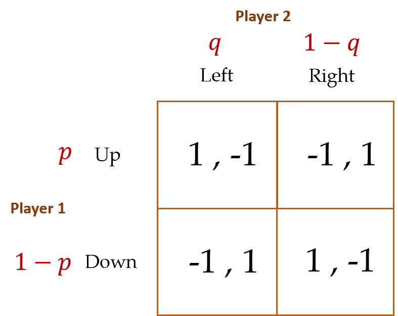
Now we suppose that Player 1 chooses Up with probability  (and thus, Down with probability
  ) and Player 2 chooses Left with probability
  (and Right with probability
  ). It turns out this game’s MSE occurs when (1) Player 1 chooses such that Player 2 is indifferent between choosing Left or Right (i.e., Player 2’s expected payoff from choosing Left equals her expected payoff from choosing Right), and (2) Player 2 simultaneously chooses such that Player 1 is indifferent between choosing Up or Down (i.e., Player 1’s expected payoff from choosing Up equals his expected payoff from choosing Down). In particular:
Player 1 chooses such that:
 .
.
Player 2 similarly chooses such that:
 .
.
Thus, Player 1 (as a member of Homo economicus) chooses Up half the time, and Player 2 (also a member of Homo economicus) chooses Left half the time. Probably the best way each player can be true to their respective strategies is to flip a fair coin (e.g., for Player 1, it might be “Heads I go Up, tails I go Down,” and similarly for Player 2).
Let’s see why the equality  holds when Player 2’s expected payoff from choosing Left equals her expected payoff from choosing Right (you’ll then be able to see why
  holds when Player 1’s expected payoffs from choosing Up and Down are equated). When Player 2 chooses Left and Player 1 chooses Up, Player 2’s payoff is -$1. The probability of Player 1 choosing Up is , hence Player 2’s expected payoff from choosing Left, conditional on Player 1 choosing Up, is $
 . Similarly, when Player 2 chooses Left and Player 1 chooses Down, Player 2’s payoff is $1. The probability of Player 1 choosing Down is , hence Player 2’s expected payoff from choosing Left, conditional on Player 1 choosing Down, is $
 . We then sum these two values (i.e., $ plus $) to attain Player 2’s (unconditional) expected payoff from choosing Left. The same process is followed to determine Player 2’s expected payoff from choosing Right. Setting these two expected payoffs equal solves for
  .[9]
.[9]
The proof for why an MSE is determined by each player randomizing their choice such that the expected payoffs for the other player are equated across that player’s choices is simply proved by contradiction. If, for example, Player 1 randomizes his choices such that Player 2’s expected payoff is larger when she chooses Left than Right (i.e., because Player 2 can see that  ), Player 2 will always choose Left. Because he more often chooses Down when , Player 1’s payoff is lower than it otherwise would be if he instead chose = 1.[10] The same logic holds when Player 1 chooses
  , in which case Player 2 always chooses Right. Because he more often chooses Up when , Player 1’s payoff is again lower than it otherwise would be if he instead chose = 1. This is because Player 1’s payoff is again guaranteed to be -$1 when . Thus, the best Player 1 can do is set = 1. The proof is the same for Player 2. Hence, we have proved why an MSE is obtained—and is the optimal outcome for this game—when each player randomizes their choice such that the expected payoffs for the other player are equated across that player’s choices. Whew!
Camerer (2003) informs us that in studies with two-choice games (i.e., games where the two players play the zero-sum game two times consecutively), Homo sapiens tend to use the same strategy after a win but switch strategies after a loss. This “win-stay, lose-shift” heuristic is a coarse version of what’s known as “reinforcement learning.” In four-choice games (players play four times consecutively), Homo sapiens’ strategies are remarkably close to MSE predictions by the fourth time they play the game.
When I was teaching in Myanmar, this was the one game I was called into service to play myself (we had an odd number of students that day). By then, I had gotten to know my students quite well individually. I was designated Player 1, and my student (I will call her Sally) was designated Player 2. We were playing a “single-choice game” due to time constraints imposed on the course. I had observed Sally over the previous weeks and concluded that she was unlikely to just flip a proverbial coin in deciding whether to choose Left or Right. She was right-handed and always sat to my right in the classroom. I guessed she would choose Right. So, I chose Down. My guess was, luckily for me, proven correct by Sally.
Afterward, when I explained my strategy to the students, I emphasized that a player need not actually randomize his moves as long as his opponent cannot guess what he will do. An MSE can therefore be an “equilibrium in beliefs,” beliefs about the likely frequency with which an opponent will choose different strategies. But I reminded the students that we had only played a single-choice game. With repeated play, chances are Sally would have begun to randomize her choices, to the point that flipping a coin would become my best strategy as well. We would slowly but surely evolve from Homo sapiens to Homo economicus.
Stag Hunt (Reprise)
In our first assessment of the Stag Hunt game, we learned that two PSEs exist, with no way of definitively determining which of the two are most likely to occur. As a result, we are compelled to determine the game’s MSE, as this is as close as we can get to identifying a unique analytical equilibrium. The game’s payoff matrix is reproduced here, this time accounting for the players’ probabilistic moves:
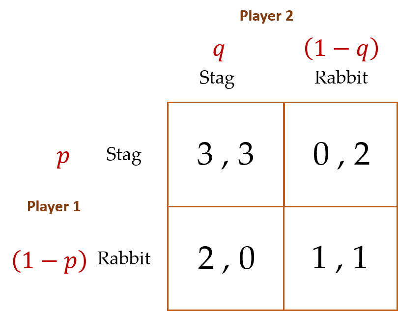
Using the same procedure as shown for determining the analytical MSE for the Zero-Sum game, the value of for Player 1 is determined as  and the value of for Player 2 is determined as
  . Each hunter might as well flip a fair coin in deciding whether to hunt stag or rabbit.
It turns out that the MSE for this game results in expected payoffs for each player that are larger than the certain payoffs obtained when both hunt rabbit (which, you’ll recall, is one of the game’s PSEs), but lower than the payoffs obtained when both hunt stag (the game’s other PSE). To see this, we can calculate Player 1’s expected payoff for the MSE as  = $1.5. Dissecting this equation, the first term is Player 1’s payoff in the (Stag, Stag) cell of the matrix multiplied by the probability that both players will choose to hunt stag (
 ). Similarly, the second term—Player 1’s payoff in the (Stag, Rabbit) cell multiplied by the probability that Player 1 chooses to hunt stag and Player 2 chooses to hunt rabbit—is equal to
  . And so on for Player 2. This is another way of saying that, when faced with the Stag Hunt, flipping a coin essentially leads to a bit less than “splitting the difference” for each player from jointly hunting stag and jointly hunting rabbit (technically speaking, splitting the difference would result in payoffs of $2 each).
Cooper et al. (1990 and 1994) used the following payoff matrix as the baseline (or what they call the Control Game (CG)) for their Stag Hunt game experiment:

A clear majority of their Homo sapiens pairs who participated in this single-choice CG game obtained the inefficient (Rabbit, Rabbit) equilibrium. The authors also had different sub-groups of subjects play what they called (1) the CG-900, where Player 1 could opt out and award both players 900 instead of playing the game (note that 900 > 800); (2) the CG-700, where Player 1 could opt out and award both players 700 instead of playing the game (note that 700 < 800); (3) CG-1W, where one of the two players is allowed to engage in “cheap talk” with the other player, presumably to nudge the other player into committing to hunt stag; and (4) CG-2W, where both players are allowed to engage in cheap talk in an effort to nudge each other into committing to hunt stag.
Cooper et al. found that 97% of player pairs chose the (Rabbit, Rabbit) PSE in the CG treatment. A large number of Player 1s also took the outside option in the CG-900 treatment. In cases where Player 1 refused the outside option, more than a supermajority of player pairs (77%) obtained the efficient (Stag, Stag) equilibrium. In the CG-700 treatment, the majority of player pairs reverted to the inefficient (Rabbit, Rabbit) equilibrium. Lastly, with one-way cheap talk between players the efficient (Stag, Stag) equilibrium jumps from 0% in the CG treatment to 53%. Unexpectedly, the jump is even greater for two-way cheap talk (up to 91%).
These results are encouraging for Homo sapiens because by simply allowing players to communicate with each other (presumably pre-committing to hunt stag), Homo sapiens are, for the most part, capable of attaining the efficient outcome where both players hunt stag together. In cases where an outside option is available for one of the players, as long as that option’s payoff is larger than the mutual payoffs associated with the (Rabbit, Rabbit) PSE, yet lower than the mutual payoffs associated with the (Stag, Stag) PSE, the player with the outside option conjectures that the other player will choose to hunt stag, who is likely to end up confirming that conjecture.
Battle of the Sexes
While it is unclear who actually named this game, there is little debate about the genesis of the title’s popularization, which occurred on Mother’s Day in 1973 at the dawn of the women’s liberation movement.[11] Tennis stars Bobby Riggs and Margaret Court faced off in a $10,000 winner-take-all challenge match, which then 55-year-old Riggs, a tennis champion from the late 1930s and 40s who was notoriously dismissive of women’s talents on the tennis court, resoundingly won. Later that year, Riggs challenged the higher-profile tennis star Billie Jean King to a $100,000 winner-take-all challenge match, which King won handily.
Although the game we have in mind here is far from being a sports match between the sexes, it does capture the flavor of challenges that sometimes bedevil couples’ coordination decisions. The payoff matrix for this game is presented below. Like the Stag Hunt, the game’s analytical equilibrium consists of two PSEs (can you identify them?). Therefore, to determine the game’s unique MSE, we acknowledge Spouse 1’s and Spouse 2’s probabilistic strategies upfront.
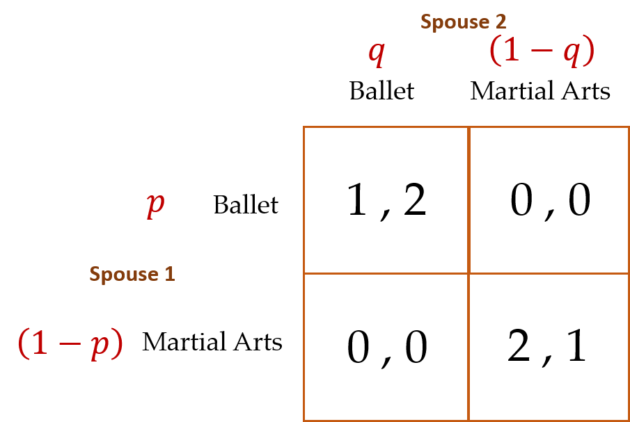
Given what you have just learned about solving for MSEs in the Stag Hunt and Zero-Sum games, you can show that for this game, = 1/3 and = 2/3. Further, the expected payoff in the MSE for each spouse is $0.67. Interestingly, these expected payoffs are lower than the least preferable payoff in either of the game’s two PSEs, where the spouses either agree to watch the martial arts performance or attend the ballet. Recall that in the Stag Game’s MSE the expected payoffs for each player “split the difference” of payoffs from the two PSEs.
In Cooper et al.’s (1989) experiments with Homo sapiens, subjects mismatched 59% percent of the time, which is actually an improvement over mismatching in the game’s analytical MSE. Mismatching occurs in the MSE when one player chooses Ballet and the other Martial Arts. This occurs  = 67% of the time. The authors also found that when one player (say, Spouse 1 in our game) is given an outside option (which, if Spouse 1 takes, pays him and his spouse some value
  , such that
  ), and the husband rejects the option, the analytical equilibrium would entail Spouse 2 surmising that Spouse 1 will then choose Martial Arts. Thus, Spouse 2 should also choose Martial Arts. In their experiment, Cooper et al. (1989) found that only 20% of Spouse 1s chose the outside option. Of the 80% of Spouse 1s who rejected the option, 90% obtained their preferred outcome—Martial Arts, here we come!
With one-way communication, the players coordinated their choices 96% of the time! However, with simultaneous two-way communication, they coordinated only 42% of the time! What happened? Recall that, in the Stag Hunt game, two-way communication enhanced coordination. Here, in the Battle of the Sexes, it has the opposite effect. Lastly, Cooper et al. (1989) found that when one of the players is known to have chosen ahead of time, but the other player is not informed about what the other player chose, the mismatch rate between the players decreased by roughly half (relative to the baseline game with no communication or outside options).
Penalty Kick
There are few team sports where an individual player is put in as precarious a position as a goalie defending a penalty kick in the game of soccer (or football if you are from anywhere else in the world except the US, Canada, Australia, New Zealand, Japan, Ireland, and South Africa). Homo sapiens rarely look more vulnerable than when put in a position of having to defend a relatively wide and high net from a fast-moving ball kicked from only 12 yards away.
Spaniel (2011) provides a nice analogy in the context of a payoff matrix where we are forgiven for taking the liberty of depicting the analytical equilibrium as an MSE upfront. Do the payoff combinations for the striker and goalie in each cell of the matrix ring a bell? The bell should be ringing zero-sum game.
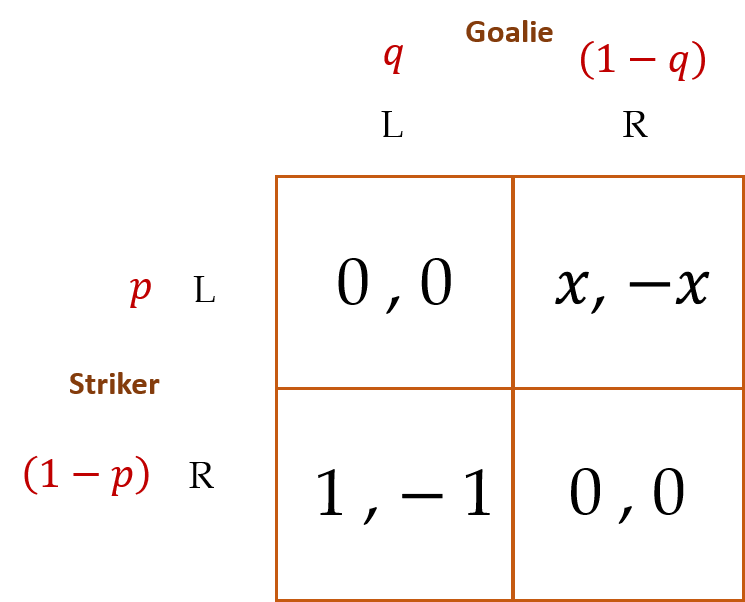
For this game, we assume a superhuman (as opposed to a mere Homo economicus) goalie. If the striker kicks Left (L) and the goalie guesses correctly and dives L, the goalie makes the save for certain. Similarly, if the striker kicks Right (R) and the goalie correctly dives R, the goalie again makes the save for certain. The striker, however, is fallible. If she kicks R and the goalie dives L, she scores for certain. But if she kicks L and the goalie dives R, she only scores with probability .
Using the method we previously developed to solve for an MSE in the Stag Hunt, Zero-Sum, and Battle of The Sexes games, verify that, in the equilibrium,  and
and  . Further, for those of you who know a little calculus, you can use these equations to solve for the respective first partial derivatives of and with respect to , as
  and
and  . Herein lies the closest thing to understanding the likely MSE choices that are made by the goalie and striker.[12]
The first partial derivatives together inform us that, in an MSE, as the striker’s probability of scoring goes up when she kicks L (embodied by an increase in ), the probability of the striker kicking L actually goes down. Analytically speaking, it is as if the striker uses one degree of iterated knowledge to determine the kick’s direction. The more the goalie believes the striker has a higher probability of scoring when she kicks L, the more likely the goalie will dive L. Thus, it makes more sense for the striker to kick R.
The next time you watch a game with lots of penalty kicks, you will be able to test this equilibrium concept in your own experiment with Homo sapiens.
Hotelling’s Game
No, this is not a game played among hoteliers. The game is named after Harold Hotelling, a 20th-century mathematical statistician and theoretical economist who pioneered the field of spatial, or urban, economics. The game is depicted below:
Suppose there are two vendors (v1 and v2) on a long stretch of beach selling the same types of fruit juices. The vendors simultaneously choose where to set up their carts each day. Beachgoers are symmetrically distributed along the beach. The beachgoers buy their fruit juice from the nearest vendor.
The line graph below distinguishes the furthest south location on the beach at 0 and the furthest north location at 1.

If you are one of the two vendors where would you decide to locate your cart on the beach?
The analytical equilibrium for this game is a PSE. The logic behind its solution goes like this:
If v1 locates at ½ she guarantees herself at least half of the total amount of business on any given day—more if v2 doesn’t also locate at ½. Indeed, v1 locating at ½ maximizes her profit. To see this, start v1 at 0 and v2 at 1. Hold v2 at 1 and move v1 toward ½. Note that v1 commands the most exposure to beachgoers at location ½. Given that v1 chooses location ½, it is in v2’s best interest to also locate at ½ (using the same logic we used to determine that v1 would locate at ½). Thus, (½, ½) is the PSE for this game.
It should be no surprise that this result is also known as the Median Voter Theory: throughout a typical campaign, candidates for public office tend to gravitate toward the middle of the political spectrum, i.e., toward the “median voter.”
Collins and Sherstyuk (2000) studied how two-, three-, and four-player Hotelling Games were played among Homo sapiens. The authors found that, in two-player games, Homo sapiens’ strategies are remarkably close to the analytical PSE prediction of (½, ½). In four-player games, the analytical PSE occurs at locations ¼ and ¾. Homo sapiens cluster at these locations, but also somewhat in the middle as well. In three-player games, the PSE occurs where each player randomizes his locational choice uniformly over the interval of locations between ¼ and ¾ inclusive, denoted [¼, ¾]. Thus, location intervals [0, ¼) and (¾, 1] are avoided. In three-player games, relatively smaller percentages of players locate outside the PSE interval of [¼, ¾] and larger percentages of players locate within the PSE interval—way to go Homo sapiens! Homo economicus would have located strictly within the PSE interval, with each player randomizing his choice uniformly over the PSE interval.
Is More Information Always Better?
The rational-choice model of Homo economicus answers “yes”, in most cases. The more information the better—more information can aid a consumer’s decision-making. But wait. Spaniel (2011) offers a game where the answer is surprisingly “no,” more information is not always better, even for Homo economicus.
Consider the following game: Player 1 chooses whether to play or not. If Player 1 chooses not to play, both Players 1 and 2 get $100. Simultaneously to Player 1’s choice, Player 2 chooses between Heads (H) and Tails (T) on a coin flip, or chooses not to gamble on the coin flip. If Player 1 had chosen to play and Player 2 had chosen not to gamble on the coin flip, both players receive $200. If instead Player 2 chooses to gamble, the coin is flipped. If Player 2 has called the outcome of the flip correctly, she wins $300 and Player 1 loses $300; vice-versa if Player 2 has called the outcome of the flip incorrectly. Therefore, the game looks like this:
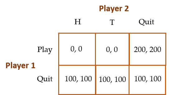
Note that the (0,0) payoffs in the cells (Play, H) and (Play, T) represent the players’ respective expected payoffs since whether the players win or lose $300 depends upon Player 2’s 50-50 luck in correctly predicting the outcome of the coin flip. The analytical equilibrium for this game goes as follows:
Because Player 2’s weakly dominant strategy is to Quit, the PSE for this game is for Player 1 to choose Play and Player 2 to choose Quit (i.e., (Play, Quit)). Note that this equilibrium is efficient! Most importantly for our purposes, Player 2 gets $200 in this equilibrium.
Now we consider a slight tweak to this game where Player 2 has private information about the outcome of the coin flip before he decides whether to play or quit. In other words, Player 2 now knows whether the coin has come up Heads or Tails beforehand. Thus, Player 2 is assured of winning $300 if Player 1—who has no prior knowledge of the outcome of the coin flip—decides to Play. The key question is whether Player 1 will now choose Play with positive probability (i.e.,  ). If not, then Player 2 has been harmed by having private information about the outcome of the coin flip—he wins only $100, instead of $200.
Recall that, in the previous game, Player 2 chose whether to play or quit before the coin was flipped. She was, therefore, uninformed about the outcome of the coin flip before deciding whether to play the game. Now, suppose Player 2 chooses whether to play or quit after the coin is flipped, and that the outcome of the coin flip is Player 2’s “private information.” The players are now involved in what’s known as a “Bayesian Nash Game,” where there are effectively two types of Player 2’s—an H type (with a probability of = 0.5 and a T type (with a probability of (1 – ) = 0.5. The game now looks like:
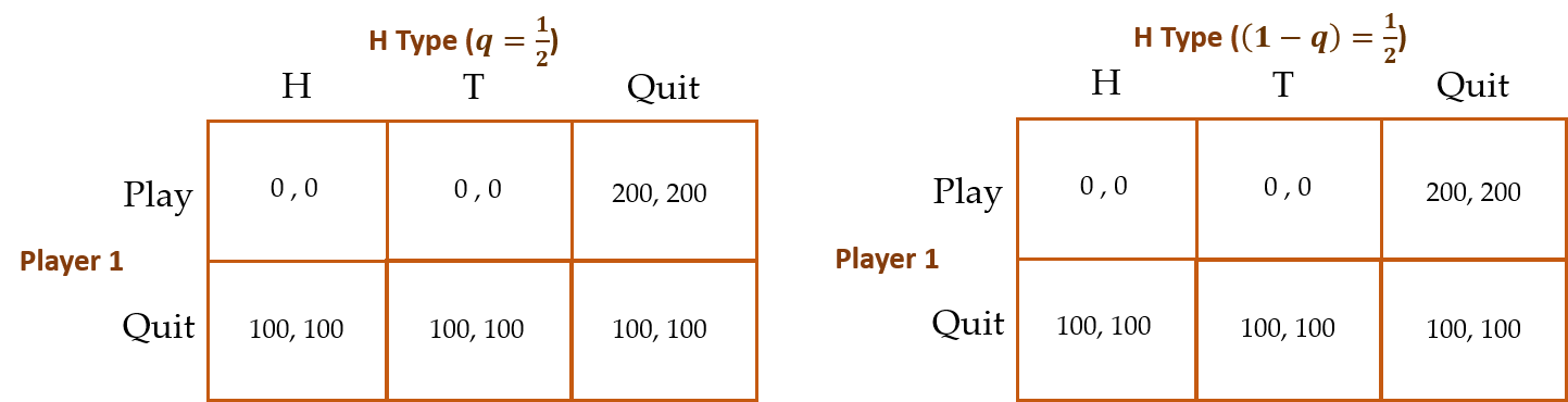
The analytical equilibrium goes as follows:
Unfortunately for Player 2, Player 1 will set = 0. If Player 1 sets , then Player 2 will simply play the correct side of the coin—H if it was H and T if it was T—thus ensuring a win of $300 when Player 1 Plays and winning $100 when Player 1 Quits. But then, Player 1 “wins” -$300 when she Plays, implying that Player 1 will never choose to Play (i.e., she will never choose ). Thus, the analytical equilibrium for this game is (Quit, Quit) with each player winning $100.
Since $100 is less than what Player 2 won when he did not possess private information about the outcome of the coin flip (which was $200), more information in this context is not better for either player. I don’t know about you, but there are plenty of instances where having less information to sift through before making a decision eases my mind and actually makes me feel happier. For example, I tend to assemble appliances, furniture, or equipment with much less angst when the instructions are concise and to the point, preferably accompanied by clear pictures or diagrams for me to follow. Lengthy written descriptions often prey upon my insecurities and impatience.
Market Entry
Consider the following game proposed by Camerer (2003):
Each of 20 players decides privately and anonymously whether to enter or stay out of the market. For each period, a different “market carrying capacity,” denoted by odd integer  (1, 3, 5, 7, 9, 11, 13, 15, 17, 19), is publically announced, after which the players make their entry decisions into the market.
Each player’s payoff ( ) is calculated as:

where  = $100,
  = $2, and
  represents the total number of players who enter the market. Note that at the time of their decisions, each player knows the values of , ,
  , and
, and  = 20, but obviously not .
Example: If = 7, and in equilibrium = 4, a player who decided not to enter the market that period receives $100, and a player who entered the market receives 100 + (2 x 3) = $106.
As Camerer (2003) shows, the analytical equilibrium for this game is rather complicated.
At the market level, there are two Nash Equilibria per value of :
- = . For example, let = 7. If = 7, then each of the 20 players earns $100. If one of the seven entrants instead chooses to stay out of the market, then she will not increase her payoff above $100 (she now earns $100 as a non-entrant). If, instead, one of the game’s 13 non-entrants decides to enter the market, this new entrant will decrease her payoff from $100 to $98. Thus, no player has a “profitable deviation” from this equilibrium.
- =
 . For example, let = 9 . If = 8, then each of the eight entrants earns $102, and each of the 12 non-entrants earns $100. If one of the eight entrants instead chooses to stay out of the market, she will decrease her payoff by $2 (from $102 to $100). If one of the game’s 12 non-entrants decides to enter the market, then this new entrant’s payoff remains $100 (since now = = 9). Thus, again no player has a profitable deviation from the equilibrium.
At the individual player level, there is a unique MSE. Letting  represent the probability of any given player deciding to enter the market for a given , and letting represent the total number of players, a given player’s expected payoff from entering is calculated using the expression for the binomial distribution,

For background on the binomial distribution see,
http://onlinestatbook.com/2/probability/binomial.html.
Thus, an individual player reaches the MSE when,

( i.e., when the player is indifferent between entering the market (expected payoff represented by the left-hand side of the equality) and staying out of the market (certain payoff represented by the right-hand side of the equality), which can be solved for
![p\left(c\right)=\frac{\left[r\left(c-1\right)+k-v\right]}{r\left(n-1\right)}](https://uen.pressbooks.pub/app/uploads/quicklatex/quicklatex.com-c654652ae342b6afac4e076eeb2add77_l3.png "Rendered by QuickLaTeX.com") .
.
Thus, in equilibrium,
![m=np\left(c\right)=\frac{n\left[r\left(c-1\right)+k-v\right]}{r\left(n-1\right)}](https://uen.pressbooks.pub/app/uploads/quicklatex/quicklatex.com-7590820c25383ea87eab12e890d84306_l3.png "Rendered by QuickLaTeX.com") .
.
In their laboratory experiments, Sundali et al. (1995) found that Homo sapiens mimic the analytical equilibrium rather closely. In a baseline setting (Experiment 1), 20 subjects were provided with no feedback between 60 rounds of play—a series of six blocks, each block based upon a randomly chosen value of  , were played by each subject 10 times each.[13] In the first block, one of the 20 subjects chose to enter the market ( = 1 ) when = 1, four subjects entered ( = 4 ) when = 3, seven entered ( = 7 ) when = 5, and so on.
Sundali et al. ultimately find a relatively close correspondence between the mean values of and their associated values of across the six blocks. Recall that in the analytical equilibrium  (i.e., and should be roughly equal). This close correspondence is supported by relatively large (close to one) correlation coefficients reported for each block (with a coefficient of 0.92 for the 60 rounds in total). This means that on average and moved in roughly the same direction over the 60 rounds—when was a relatively large value, so was , and when was relatively small, so was (0.92
  1, where 1 implies perfect linear correlation between the two values). Second, variability in the market entry decision across participants was largest for intermediate levels of .
In a second experiment (Experiment 2), subjects were provided with feedback at the end of each round regarding the equilibrium value of , as well as their respective payoffs for each round and cumulative payoffs up to the round. Subjects were also encouraged to write down notes concerning their decisions and outcomes. Results for this experiment were even closer to those predicted for Homo economicus in the analytical equilibrium.
As Camerer (2003) points out, how firms coordinate their entry decisions into different markets is important for an economy. If there is too little entry, prices are too high and consumers suffer; if there is too much entry, some firms lose money and waste resources, particularly if fixed costs are unsalvageable. Public announcements of planned entry could, in principle, coordinate the right amount of entry, but announcements may not be credible because firms that may choose to enter have an incentive to announce that they surely will do so in order to ward off competition. Government planning may help reduce this perverse incentive, but governments are nevertheless vulnerable to regulatory capture by prospective entrants seeking to limit competition. Evidence from the real world often suggests that too many firms choose to enter markets in general, particularly in newly forming markets. As we learned in Section 1, the phenomenon of excessive entry could reflect a Confirmation Bias on the part of potential entrants, leading to overconfidence in their abilities to obtain positive profits.[14]
Weakest Link
Consider the following game presented in Camerer (2003):
Players (more than two) pick numbers from 1 to 7. Payoffs increase with the minimum of all the respective numbers chosen, and decrease with the deviation of their own choice from the minimum. The specific payoffs (in dollars) for our game are shown in the table below:
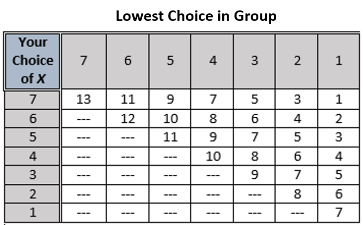
For example, if a player chooses 4 and the minimum chosen by another player in the group is 2, then that player’s payoff is $6.
You may recognize this game as being a generalization of the Stag Hunt and reminiscent of the Continental Divide. As such, there is an efficient equilibrium where each player chooses the number 7, and an inefficient, risk-dominant equilibrium where each player plays it safe by choosing the number 1. Choices of 5 and 6 act as potential basins of attraction for 7, while choices of 2 and 3 are potential basins of attraction for 1.
Van Huyck et al. (1990) played this game with a total of 107 Homo sapiens parcelled into groups consisting of between 14 and 16 subjects for 10 rounds. The authors found that relatively large numbers of the subjects choose higher numbers in the first round—33 players chose the number seven, 10 players chose the number six, 34 chose five, and 17 chose 4. However, by the tenth and final round, 77 players chose the number one and 17 chose the number 2. These results are obviously discouraging. Recall that the efficient equilibrium is where there is no weak link among the players—every player chooses the number seven, and no players choose the number one.
Interestingly, results for 24 Homo sapiens who played the game for only seven rounds were more encouraging. In the first round only 9 players chose number seven, zero chose number 6, and four chose number 4. By the seventh and final round, 21 had chosen the number seven.
Perhaps these results are unsurprising given what we’ve already learned about Homo sapiens’ behavior in the Finitely Repeated Trust (Centipede) Game. In that game, we learned that in repeated play, trust and trustworthiness between two players can be achieved, at least temporarily. Random re-matching obviates the build-up of trust and trustworthiness that can arise through repeated play. And, generally speaking, it is more difficult to build trust and trustworthiness among a larger group of players.
As for real-world applications of the Weakest Link Game, Camerer (2003) points out that in the airline business, for example, a weakest link game is played every time workers prepare an airplane for departure. The plane cannot depart on time until it has been fueled, catered, checked for safety, passengers have boarded, and so on. For short-haul carriers, which may use a single aircraft on multiple flights daily, each departure is also a link in the chain of multiple flights, which creates another weakest link game among different ground crews.[15]
Weakest Link with Local Interaction (Two Versions)
We now consider two different versions of the Weakest Link Game presented in Camerer (2003). In the first version, players are provided with some information at the end of each round about the choices made by the other players. In the second version, players play separate games simultaneously with their neighbors, thus permitting the experimenter to test whether spatiality might affect the game’s equilibrium outcome among Homo sapiens.
Here is version one:
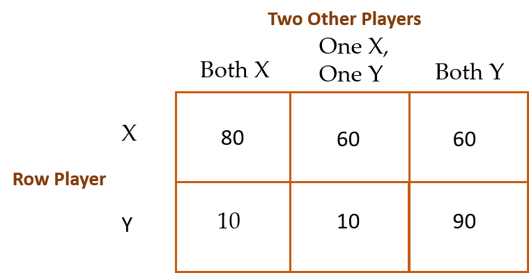
To begin, players individually choose the letter X or Y in separate groups of three players each over 20 rounds. Payoffs (in dollars) are shown in the table below. Each player learns the two choices made by the other two players at the end of each round (but not which player made with choice).
And here is version two:
In this version of the game, players face the same payoff matrix:
But each group of eight players is arranged in a circle, and each subject plays with his two other nearest neighbors:
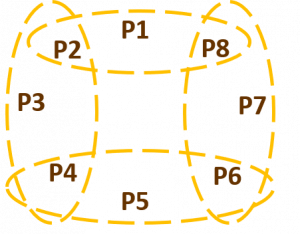
For example, in this diagram Player P1 plays with Players P2 and P8 directly, while Player 2 simultaneously plays with Players P3 and P4 and Player P8 simultaneously plays with Player P6 and P7.
Note that the risk-dominant, inefficient equilibrium in both versions occurs when each player decides to play it safe by choosing option X. The efficient equilibrium occurs when all three players in a group choose Y. In this way, the game mimics the Weakest Link Game introduced earlier. In keeping with Van Huyck et al.’s (1990) original findings, we would therefore expect that, because the game here is being played in relatively small groups (three players per group), Homo sapiens playing these games would again mimic Homo economicus and obtain the efficient equilibrium, especially in version one of the game. Version two presents a complication since, although the groups are small, each player now plays with multiple sets of different players simultaneously, either directly or indirectly. The even-numbered players do so directly (e.g., Player P2 simultaneously plays with Players P1 and P8, on the one hand, and Players P3 and P4 on the other). Odd-numbered players do so indirectly (e.g., Player P1 plays with Players P2 and P8, who in turn play simultaneously with Players P3 and P4 and Players P6 and P7, respectively).
In playing this game with different groups of Homo sapiens, Berninghaus, et al. (2002) found that in standard (non-circular) three-person groups, players initially play Y about three-quarters of the time—specifically, in their experiments seven out of eight groups of three players coordinated on the efficient (all-Y) equilibrium. No surprise. However, in the local-interaction (circular) groups, players started by playing Y only half of the time, but then play of Y fell steadily to almost none by the 20th round of the game. Specifically, players responded to their neighbors by playing X 64% of the time when one other neighbor had chosen X. The authors likened this result to the spread of a disease through a population by close contact—in this case, the spread of fear. The incidence of playing X spreads from neighbor to neighbor, eventually infecting the entire group.
A merger where one or more disparate groups of individuals merge into a single group is an extreme form of local interaction, one that is continually played out through history on a macro-scale (e.g., beginning with families merging into clans who merge into ethnic groups, to villages and city-states to nation-states and sometimes empires). On a micro- scale, mergers occur when one company acquires another and becomes its “parent company.” Mergers and acquisitions among businesses are a common feature of market economies—some would say they pose a threat to competition, while others believe they can provide efficiency gains via economies of scale.
Camerer and Knez (1994) wondered how the Weakest Link game might inform us about the efficacy of mergers occurring between two small groups into a single larger group. The group-size effect noted earlier suggests that, all else equal, larger (merged) groups would be less likely to converge to the efficient equilibrium where all group members individually select the number seven. This is exactly what Camerer and Knez found. Interestingly, the provision of public information (to each group about the other group with which it later merged) appears to have worsened the outcomes (i.e., increased the inefficiency) in paired small groups of three players each.
Camerer and Knez conclude that the results for merged groups in the context of a Weakest Link game are not encouraging. However, not to be outdone by these unflattering results, the authors added another treatment to the mix (in addition to the provision of public information about the performance of the other groups in the previous round). The additional treatment was a public announcement to all groups of a “bonus” if everyone picked the number 7 (i.e., if each merged group chose the Pareto efficient outcome). Thankfully, the announcement nudged the merged groups immediately in round 1, from 90% choosing numbers one or two to 90% choosing number 7. Camerer and Knez’s Homo sapiens apparently need a little added incentive post-merger to attain an efficient equilibrium in their weakest-link choices.
Concluding Remarks
Section 3 has introduced you to the burgeoning field of behavioral game theory, a field that investigates how Homo sapiens play several of the classic games devised by game theorists to depict expected outcomes (i.e., analytical equilibria) when people interact in a variety of social situations. In particular, behavioral game theory identifies how Homo sapiens deviate from a game’s analytical equilibrium and devises tweaks to the game in an effort to gain insight into what might be causing the deviation.
We began our exploration of the field in Chapter 7 by studying the classic bargaining games—Ultimatum Bargaining, Nash Demand, and Finite-Alternating Offers. The distinguishing features of these games are (1) they are played sequentially (i.e., one player makes a choice first and then the other player chooses); (2) the analytical equilibrium is premised upon each player thinking ahead about the other player’s subsequent move before choosing what to do presently (i.e., each player thinks iteratively); and (3) the process of thinking iteratively requires that each player first considers what she should choose to do in the game’s final stage, and then work backward to what to do in the game’s initial stage. The resulting equilibrium is known as “subgame perfect” solved via “backward induction” and reflective of an “iterated dominance” in the player’s respective strategies. As complicated as all of this sounds, we learned that Homo sapiens often achieve this type of equilibrium in a variety of contexts.
Likewise, we studied a variety of multiple-stage games with subgame perfect equilibria involving sequential moves by the players, each in their own way demonstrating the concept of iterated dominance. Recall the Escalation, Burning Bridges, Police Search, Dirty Faces, and Trust Games. In the Dirty Faces game, the trajectory toward the game’s analytical equilibrium depends upon an initial, random draw of cards. One draw quickly leads players to the equilibrium; the other draw necessitates more intensive “iterated knowledge” on the part of the players. As expected, Homo sapiens do a better job of attaining the equilibrium when less iterated knowledge is required of them. In the Trust game, Homo sapiens players demonstrate excessive trust and insufficient trustworthiness.
Next, we considered a series of games in this chapter where players are again expected to use iterative thinking but this time in contexts where decisions are made simultaneously, not sequentially. As a result, players are expected to use “forward induction” in predicting how their opponents will play rather than backward induction. In some of these games, the analytical equilibria exist in “pure strategies,” where the payoffs are structured in such a way as to make non-cooperative strategies “dominant” over others and the corresponding equilibria inefficient. This was the case with the famous Prisoner’s Dilemma where, unfortunately, Homo sapiens tend to mimic self-interested Homo economicus and obtain the inefficient equilibrium. However, when Homo sapiens are allowed to play the game repeatedly, cooperation among players ensues.
Other simultaneous games do not exhibit dominant strategies, leading instead to “mixed-strategy” equilibria where players choose their strategies randomly but in accordance with some rule, such as flipping a fair coin. The Stag Hunt, Zero-Sum Game, and Battle of The Sexes are examples of games with mixed-strategy equilibria. Empirical research suggests that Homo sapiens are capable of attaining a games’ mixed-strategy equilibrium, but only with the aid of additional incentives such as one- or two-way communication (known as “cheap talk”) among players, or the availability of “outside options” for one of the players that the other player is also aware of. Similar results were found for other simultaneous-move games such as the Market Entry and Weakest Link Games. In the Market Entry Game, Homo sapiens responded to both previous-round and cumulative feedback by more closely mimicking the analytical equilibrium. In Weakest Link Games, smaller player groups achieved the analytical equilibrium more often. But when players played two games simultaneously—each game with a different set of players—the analytical equilibrium was obtained less often.
Therefore, it appears that Homo sapiens tend to perform more like Homo economicus in social settings (i.e., in games played with multiple players) than in individual settings (e.g., the laboratory experiments presented in Section 2), particularly when appropriate incentives are provided in the social setting. Homo sapiens tend to learn in both settings through repeated play and with appropriate incentives. For example, with appropriate incentives, if the opt-out payoffs are set too low or too high, players with access to opt-out options are more likely to choose strategies that deviate from the analytical equilibrium. This has been demonstrated in Stag Hunt games. As we learned from experiments with Ultimatum Bargaining and the Beauty Contest, the level of a game’s stakes itself does not generally influence the probability that players will attain an analytical equilibrium.
As we proceed to Section 4, recall that the experiments and games we have studied in Sections 1–3 have traditionally been conducted with relatively small samples of university students. As such, the generalizability of their results to wider populations is justifiably drawn into question. In Section 4, we explore empirical studies based upon larger and more diverse (i.e., more “representative”) samples of individuals, the results from which are, by design, more generalizable to wider populations.
Study Questions
Note: Questions marked with a “†” are adopted from Just (2013), those marked with a “‡” are adopted from Cartwright (2014), and those marked with a “ ” are adopted from Dixit and Nalebuff (1991).
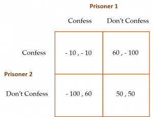
- † Consider the Prisoner’s Dilemma game depicted below in which two prisoners are accused of a crime. Both are isolated in the prison. Without a confession, there is not enough evidence to convict either. A prisoner who confesses will be looked upon with lenience. If one prisoner confesses and the other does not, the prisoner not confessing will be imprisoned for a much longer time than if she had confessed. The payoffs for the prisoners are depicted in the matrix below (Prisoner 1’s payoffs are to the right of the comma in each cell, and Prisoner 2’s are to the left of the comma in each cell). (a) If a selfish prisoner plays this prisoner’s dilemma against an opponent she believes to be altruistic, what will her strategy be? (b) Now suppose the prisoner’s dilemma is played three times in sequence by the same two prisoners. How might a belief that the other prisoner is altruistic affect the play of the selfish prisoner? Is this different from your answer to part (a)? What has changed?
- In discussing strategies for a finitely repeated Prisoner’s Dilemma game, it was mentioned that “tit-for-tat” may be a strategy that induces cooperation among players in an infinitely repeated version of the game. Recall that a player adopts a tit-for-tat strategy when he cooperates in the first round of the game and then, in each successive period, mimics the choice (deviate or cooperate) made by his opponent in the previous period. Thus, if Player 1 plays tit-for-tat and Player 2 deviates in the first round, then Player 1 commits to deviating in the second round, and so forth. If Player 1 believes that Player 2 is also playing tit-for-tat, and the game’s payoff matrix is the same as that originally presented in this chapter (repeated below for reference), is it still in Player 1’s interest to play tit-for-tat? Explain.
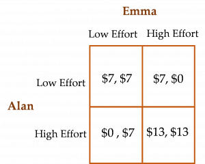
- ‡ Consider the game below, played between Alan and Emma. Alan’s payoffs are represented by the first dollar value in each cell of the matrix, and Emma’s payoffs are represented by the second dollar value. Identify each of this game’s equilibria. Which equilibrium would you prefer Alan and Emma to reach together? What incentive might you give Emma and Alan to ensure that they would reach the preferred equilibrium?
- Choose a simultaneous game you learned about in this chapter. In what way would permitting communication between the players before the game begins affect the game’s outcome?
- In the discussion of the Public Good game, it was mentioned that a Provision-Point Mechanism has been found in experiments to increase contributions to public goods. Explain why this is the case.
- ‡ Describe the similarities and differences between the Weakest Link and Threshold Public Good games, where the threshold in the public good game is a provision-point mechanism.
- Is reaching an international agreement on the control of climate change similar to a Stag Hunt game? Explain.
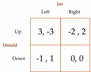
- Suppose Joe and Donald face the Zero-Sum game presented below. Calculate the game’s mixed-strategy equilibrium.
- Recall that in Cooper et al.’s (1989) Battle of the Sexes experiments with Homo sapiens, when one of the two players is allowed to communicate with the other player (i.e., there is “one-way communication”) the players coordinate their choices 96% of the time! However, with simultaneous two-way communication between the two players, they coordinate only 42% of the time! Explain what happened.
- We demonstrated how to solve for the Penalty Kick game’s mixed-strategy equilibrium. Suppose you were new to the game of soccer (or football) and assigned to play the goalie position. After watching the following YouTube video, what strategy might make the most sense for you to adopt on penalty kicks: https://www.youtube.com/watch?v=3yWZZR9ZodI.
- The map below identifies (with red markers) the locations of gas stations in Salt Lake City, Utah (Utah’s capital city). Do these gas station locations depict a pure strategy equilibrium for the Hotelling Game? Explain.

- In this chapter, we learned that when an individual acquires private information about something, this added information does not necessarily make the individual better off. In particular, when an individual (say, Player 1) acquires private information about something of common interest to both himself and another individual (say, Player 2), and Player 2 knows Player 1 has acquired this private information, Player 1 could actually be made worse off as a result of Player 2 changing her strategy in response to the fact that she knows Player 1 now has additional information. Whew! Can you think of a real-life example where the acquisition of private information actually makes the now-better-informed individual worse off? For inspiration in formulating your answer, consider watching this trailer of the 2019 movie The Farewell: https://www.youtube.com/watch?v=RofpAjqwMa8.
- Analyze this excerpt from the British game show Golden Balls in the context of something you have learned about in this chapter: https://www.youtube.com/watch?v=S0qjK3TWZE8.
- This question demonstrates how one player can turn a disadvantage encountered in a simultaneous-move game into an advantage by making a prior public announcement and thereby transforming the simultaneous-move game into a sequential-move game. To show this, suppose the players’ payoff matrix is as shown below. (a) Determine this game’s analytical equilibrium in pure strategies (i.e., its PSE). (b) Explain why Player 1 is not happy with this equilibrium. (c) Suppose Player 1 decides to preempt this game’s equilibrium outcome by announcing what his effort level will be before Player 2 decides on her effort level. Describe this new game in its extensive form (i.e., in the form of a decision tree). Using iterated dominance, identify the equilibrium for this game. Did Player 1’s preemptive announcement work to his advantage (i.e., did Player 1 give himself a first-mover advantage)? Explain. (d) Explain why Player 1’s preemptive announcement does not necessarily have to be considered credible by Player 2 to have its beneficial effect on Player 1.
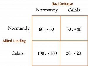
- In 1944, the Allies were planning their liberation of Europe while the Nazis planned their defense. The Allies were considering two possible landing sites—the beaches of Normandy or Pas de Calais. Calais was considered more difficult to invade but more valuable to win given its proximity to Belgium and Germany. Suppose the payoff matrix facing the Allies and the Nazis is as depicted below. (a) What type of game does the payoff matrix represent? (b) Calculate the game’s mixed-strategy equilibrium. Is this equilibrium consistent with what actually occurred in 1944? Explain. (c) Calculate the Allies’ expected payoff from following its equilibrium strategy.
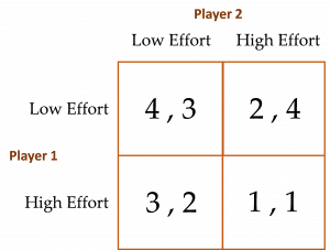
- Suppose two players are involved in a game where one of the player’s payoffs (both when she cooperates and deviates) are much larger than the other player’s (e.g., because the player with the larger payoffs (say, Player 1) is a much larger producer than Player 2). The payoff matrix for this game is provided below. Determine this game’s analytical equilibrium. Comment on this equilibrium in relation to the standard analytical equilibrium obtained in the Prisoner’s Dilemma.
Media Attributions
- Figure 1 (Chapter 8) © Arthur Caplan is licensed under a CC BY (Attribution) license
- Figure 2 (Chapter 8) © Fehr and Gachter; 2000 American Economic Association is licensed under a All Rights Reserved license
- Figure 3 (Chapter 8) © Fehr and Gachter; 2000 American Economic Association is licensed under a All Rights Reserved license
- Figure 4 (Chapter 8) © Arthur Caplan is licensed under a CC BY (Attribution) license
- Figure 5 (Chapter 8) © Arthur Caplan is licensed under a CC BY (Attribution) license
- Figure 6 (Chapter 8) © Arthur Caplan is licensed under a CC BY (Attribution) license
- Figure 7 (Chapter 8) © Arthur Caplan is licensed under a CC BY (Attribution) license
- Figure 8 (Chapter 8) © Arthur Caplan is licensed under a CC BY (Attribution) license
- Figure 9 (Chapter 8) © Arthur Caplan is licensed under a CC BY (Attribution) license
- Figure 10 (Chapter 8) © Arthur Caplan is licensed under a CC BY (Attribution) license
- Hotellings Game Figure © Arthur Caplan is licensed under a CC BY (Attribution) license
- Is More Information Always Better Figure © Arthur Caplan is licensed under a CC BY (Attribution) license
- Is More Information Always Better Figure (second figure) © Arthur Caplan is licensed under a CC BY (Attribution) license
- Weakest Link Figure © Arthur Caplan is licensed under a CC BY (Attribution) license
- Weakest Link With Local Interaction Figure v1 © Arthur Caplan is licensed under a CC BY (Attribution) license
- Weakest Link With Local Interaction payoff matrix v2a © Arthur Caplan is licensed under a CC BY (Attribution) license
- Weakest Link With Local Interaction eight player schematic © Arthur Caplan is licensed under a CC BY (Attribution) license
- Figure for Study Question 1 (Chapter 8) © Arthur Caplan is licensed under a CC BY (Attribution) license
- Figure for Study Question 3 (Chapter 8) © Arthur Caplan is licensed under a CC BY (Attribution) license
- Figure for Study Question 8 (Chapter 8) © Arthur Caplan is licensed under a CC BY (Attribution) license
- Figure for Study Question 12 (Chapter 8) © Arthur Caplan is licensed under a CC BY (Attribution) license
- Figure for Study Question 14 (Chapter 8) © Arthur Caplan is licensed under a CC BY (Attribution) license
- Figure for Study Question 15 (Chapter 8) © Arthur Caplan is licensed under a CC BY (Attribution) license
- Figure for Study Question 16 (Chapter 8) © Arthur Caplan is licensed under a CC BY (Attribution) license
- As we have learned thus far, games where players move sequentially are generally depicted as decision trees (or, in "extensive form"). In contrast, games where players move simultaneously are generally depicted as payoff matrices (or, in "strategic form"). ↵
- Game theorists make a distinction between “strictly” dominant strategies and “weakly” dominant strategies. In the Prisoner’s Dilemma, the strategies are strictly dominant because (1) the payoff of choosing Deviate when the other player Deviates ($2) is greater than choosing Cooperate ($1), and (2) the payoff of choosing Deviate when the other player chooses Cooperate ($6) is also greater than choosing Cooperate ($4). If either (not both) of these values were equal to each other (e.g., the $2 payoffs in the (Deviate, Deviate) cell were instead equal to $1 each, or the $4 payoffs in the (Cooperate, Cooperate) cell were instead equal to $6 each), then the Deviate strategy would only be weakly dominant. ↵
- Poundstone (1992) provides the onomatology of the title Prisoner’s Dilemma. As the title suggests, Prisoner’s Dilemma was used to describe a fictional game where two suspects are apprehended, and the investigator wants both to individually confess to having participated in a crime. The investigator sets the prison sentences associated with confessing (Deviate) and maintaining innocence (Cooperate) such that the suspects’ dominant strategies are to confess. ↵
- In a more recent experiment, where players engage in what they interpret as an infinitely repeated Prisoner's Dilemma game, Kim (2023) finds that higher discount factors (as a result of week- or month-long delays in when players are allowed to recoup their payoffs) induce more cooperation among the players. ↵
- In an intriguing cross-cultural comparison of the effectiveness of punishment in finitely repeated public good games, Gächter et al. (2010) find a surprising result regarding the punishment of above-average contributors. For example, in the Australian city of Melbourne and the European cities of Bonn, Nottingham, and Copenhagen, there is little punishment for above-average contributors, while in the Saudi Arabian city of Riyadh, the Greek city of Athens, and the Belarusian city of Minsk, above-average contributors were punished at the same levels as below-average contributors. The authors call this latter form of retribution anti-social punishment, attributed to their observation of a strong correlation between punishment received in one period and that doled out in the next. For example, if above-average Sam punished below-average Sally in period 1, Sally then punished Sam in period 2 as revenge. Because anti-social punishment is ultimately associated with less cooperation among players, this study’s findings serve as a cautionary tale for those who espouse punishment as a universal remedy to the free-riding problem. ↵
- With their laboratory experiments, Chan et al. (2002) sought to answer the question of whether involuntary transfers for the provision of a public good, such as taxation, crowd out voluntary transfers (i.e., private donations) that reflect a “warm-glow” emotion among subjects. The authors do not find evidence of complete crowding out in general, but suggest that crowding out increases as the rate of taxation increases. Sufficiently large rates of taxation offset the benefits of warm-glow giving. ↵
- Vilfredo Pareto was a 19th – 20th-century Italian engineer, sociologist, political scientist, philosopher, and economist. He made several important contributions to economics, particularly concerning the study of income distribution and analysis of individuals' choices. He is considered one of the fathers of welfare economics. ↵
- As with the Prisoner’s Dilemma and Stag Hunt games, environmental and resource economists recognize that the global fight against climate change exhibits features of a zero-sum game. All else equal, whenever one country invests in abating its carbon emissions, all other countries gain by not having to expend funds themselves to get the same amount of reduced carbon emissions. In terms of who bears the opportunity cost of the investment, this is one country’s loss (or at least attenuated gain) and every other country’s gain (since units of carbon reduced anywhere on the planet reduce the atmospheric stock of carbon that is responsible for rising ground temperatures and other meteorological changes occurring across the planet). ↵
- To be clear, the MSE for the zero-sum game does not always result in
 . To see this, calculate the equilibrium values for and when the payoff matrix is something like (Up, Left) = (3,-3), (Up, Right) = (-2,2), (Down, Left) = (-1,1), and (Down, Right) = (0,0). ↵
 - This is because Player 1’s payoff is guaranteed to be -$1 when . ↵
- The following interpretation is taken from history.com (2020). ↵
- Note that solving for the likelihood that a goal will actually be scored on any given penalty kick is, to put it mildly, anyone’s guess. ↵
- Thus, each subject was presented with each value of six different times over the course of the experiment. ↵
- Camerer and Lovallo (1999) designed an experiment to detect the extent to which overconfidence in one’s skills relative to what he perceives are the skills of potential competitors induces excess entry into a market and subsequent business failure. The authors uncover a phenomenon they termed reference group neglect, where excess entry is much larger when subjects participated in the experiment knowing that payoffs would depend upon skill level. These self-selected subjects neglected the fact that they are competing with a reference group of subjects who all think they are as skilled. ↵
- This suggests that efficient equilibria have been obtained in an airline company’s weakest link games if all of a passenger's connecting flights are on time. Whether or not any given passenger makes it to the airport and his connecting flights on time is his set of weakest link games. ↵
