The laboratory experiments discussed in this chapter have been designed to test the Principle and Additional Rationality Axioms presented in Chapter 3. As you will see, we Homo sapiens are rather prolific in our violations of the rationality typified by Homo economicus.

Testing the Invariance Axiom (Version 1)

Consider the following experiments designed by Kahneman and Tversky (1984):

Homo economicus would quickly determine that Program A in Experiment 1 is equivalent to Program C in Experiment 2, and Program B in Experiment 1 is similarly equivalent to Program D in Experiment 2. Thus, he would recognize that the two experiments themselves are equivalent. If each experiment were conducted separately with two different groups of Homo economicus, we would then naturally predict 50%-50% splits between Programs A and B among subjects participating in Experiment 1, and 50%-50% splits between Programs C and D among subjects participating in Experiment 2. These outcomes would be consistent with the Invariance Axiom.

To the contrary, when Kahneman and Tversky ran the experiments, 72%(28%) of the subjects in Experiment 1 chose Program A(B). The reverse occurred in Experiment 2, with 22%(78%) of the subjects choosing Program C(D). The authors surmised that this violation of the Invariance Axiom among Homo sapiens resulted from the experiments having been framed by different reference points. Experiment 1’s reference point is that people will be saved while Experiment 2’s is that people will die. This, in turn, led the Homo sapiens to make reference-dependent choices. Kahneman and Tversky identified this particular type of reference-dependency as a Reflection Effect.

Testing the Invariance Axiom (Version 2)

Kahneman and Tversky (1979) provide another test of reference-dependency and the Reflection Effect in an experiment with two groups of roughly 70 subjects each. The first group participated in the following experiment:

Since the two lotteries have the same expected values of $500, a Homo economicus with any degree of risk aversion would choose Lottery B. Of Kahneman and Tversky’s 70 Homo sapiens who participated in this experiment, 84% chose Lottery B. Not bad.

The second group of subjects participated in a slightly altered version of Experiment 1:

Note that these two lotteries are essentially identical to the two lotteries in Experiment 1. Lotteries A both give the individual a 50% chance of walking away with $2,000 and a 50% chance of walking away with $1,500. Lotteries B both ensure that the individual walks away $1,500 wealthier with certainty. Thus, any Homo economicus who would choose Lottery B in Experiment 1 should likewise choose Lottery B in Experiment 2 (or to put it another way, the percentages of Homo economicus choosing Lottery B in Experiments 1 and 2 should be equal). We would like to think that Homo sapiens will behave similarly.

Wouldn’t you know it? Of Kahneman and Tversky’s 70 Homo sapiens who participated in this experiment, only 31% chose Lottery B. What the…? This outcome led Kahneman and Tversky to conclude that their subjects were indeed making reference-dependent choices. Experiment 1 was framed in terms of winning, and the great majority of Homo sapiens responded by exhibiting risk aversion—they prefer to protect certain gains. In contrast, Experiment 2 was framed in terms of losing, and the majority of Homo sapiens responded by exhibiting risk-seeking behavior—they decided to take a gamble that was otherwise eschewed in Experiment 1. The results for Experiment 1 concur with the value function’s diminishing sensitivity to gains as described in Chapter 4, and the results for Experiment 2 concur with the value function’s diminishing sensitivity to losses.

Testing the Invariance Axiom (Version 3)

Consider the following two experiments proposed by Grether and Plott (1979):

In this case, each subject participates in both experiments. We would expect that if Homo economicus prefers Lottery A to Lottery B in Experiment 1, then she would choose to sell Lottery A for more money than Lottery B in Experiment 2. This would be consistent with the Invariance Axiom in the context of this experiment. By contrast, Grether and Plott found that 70% of the Homo sapiens who participated in the two experiments exhibited a preference reversal by choosing the relatively safe Lottery B in Experiment 1 but stating a higher selling price for risky Lottery A in Experiment 2.^[1]

A less-complicated version of Experiments 1 and 2 designed to test for preference reversal in the context of a monetary bet was tested by Tversky et al. (1990), who proposed an experiment to their students similar to the following:

The students were asked two questions: which lottery would you prefer to play, and which lottery is worth more to you (in terms of the minimum amounts of money you would be willing to accept in lieu of having the chance to play either lottery)?

We know how Homo economicus would answer. He would first calculate the expected value of each lottery ($7.50 for Lottery A and $10 for Lottery B) and then answer the two questions as “I prefer Lottery B” and “Lottery B is worth $2.50 more to me.” In other words, Homo economics would go Lottery B all the way; no preference reversal there. To the contrary, Tversky et al. (1990) found that around 75% of their subjects chose Lottery A in answer to the first question but roughly 65% of these same subjects chose Lottery B in answer to the second question. Ouch, big-time preference reversal there.

Testing the Invariance Axiom (Version 4)

Consider the following three experiments, versions of which were proposed by Kahneman (2011):

Suppose that subjects recruited to participate in these experiments are divided into two groups. One group participates in Experiments 1 and 2 simultaneously, i.e., the subjects are asked to contribute to a special fund for the Narcondam Hornbills in Experiment 1 and the farmworkers in Experiment 2. The other group participates in Experiment 3. What would we expect from two groups of Homo economicus here? If you answer that the average amounts Homo economicus subjects pledged in Experiments 1 and 2 equal the same average amounts in Experiment 3, then you’ve nailed it! Essentially, both groups are presented with the same experiments. Thus, on average, Homo economicus would violate the Invariance Axiom if the amounts pledged for Experiments 1 and 2 did not match those pledged in Experiment 3.

Kahneman hypothesizes that the average amount pledged by Homo sapiens in Experiment 1 (for Narcondam Hornbills) will exceed the average amount pledged in Experiment 2 (for the farmworkers). But in Experiment 3, the average amounts will be reversed, indicating a preference reversal.^[2]

Testing the Invariance and Dominance Axioms (Version 1)

Consider the following experiments proposed by Kahneman and Tversky’s (1984):^[3]

Begin by noting that Lottery B in Experiment 1 dominates Lottery A. This is because the expected winnings from Lottery B are greater than those from Lottery A, and the expected losses from Lottery B are less than those from Lottery A. Obviously, Homo economicus will choose Lottery B, thus not violating the Dominance Axiom.

Next comes the hard part. In Experiment 2, adding the sure win of $240 (Lottery A in Compound Lottery 1) to Lottery B in Compound Lottery 2 yields a 25% chance of winning $240 and a 75% chance to lose $760. Note that this is exactly Lottery A in Experiment 1! Similarly, adding the sure loss of $750 (Lottery A in Compound Lottery 2) to Lottery B in Compound Lottery 1 yields a 25% chance to win $250 and a 75% chance to lose $750. But this is precisely Lottery B in Experiment 1!

Thus, since Homo economicus will choose Lottery B in Experiment 1, in Experiment 2 he will choose Lottery B in Compound Lottery 1 and Lottery A in Compound Lottery 2.^[4]

What about Homo sapiens? Thankfully, none of Kahneman and Tversky’s subjects in Experiment 1 chose Lottery A, implying that Homo sapiens also abided by the Dominance Axiom. However, in Experiment 2, the great majority of subjects chose Lottery A in Compound Lottery 1 and Lottery B in Compound Lottery 2. This is the opposite of Homo economicus’ choices and demonstrates a preference reversal for these Homo sapiens (relative to their choices of Lottery B in Experiment 1). In other words, once again a majority of Homo sapiens have violated the Invariance Axiom.

Kahneman (2011) reminds us that Experiment 2 is an example of narrow vs. broad framing.^[5] Narrow framing occurs when subjects consider the two compound lotteries separately from each other  (narrowly) rather than taking the time necessary to consider the two compound lotteries jointly (broadly). Subjects who broadly frame the two compound lotteries are capable of abiding by the Invariance Axiom, i.e., all else equal, they will be more likely to choose Lottery B in Compound Lottery 1 and Lottery A in Compound Lottery 2 because they take the time to compare the two compound lotteries. As Kahneman (2011) points out, in real life broad framing induces Homo sapiens to choose high deductibles for insurance policies, eschew choosing extended warranties for the products they purchase, and not regularly check their retirement balances. Broad framing encourages adherence to “risk policies” that lead Homo sapiens to make choices with favorable odds in the long run.^[6]

Begin by noting that, just as in Version 1 above, Lottery B in Experiment 1 dominates Lottery A. This is because the expected winnings from Lottery B are greater than those from Lottery A, and the expected losses from Lottery B are less than those from Lottery A. Homo economicus chooses Lottery B and thus again does not violate the Dominance Axiom.

Next, note that Experiment 2 is effectively identical to Experiment 1. Specifically, Lotteries A in both experiments offer the same percentages of winning $0, $45,000, and $30,000, respectively, and the same percentage of losing $15,000. Lotteries B similarly offer the same percentages of winning $0 and $45,000, respectively, and the same percentages of losing $15,000 and $10,000, respectively.

Since Homo economicus chooses Lottery B in Experiment 1 via the Dominance Axiom, in Experiment 2 she will also choose Lottery B, thus abiding by the Invariance Axiom.

What about Homo sapiens? Thankfully, none of Tversky and Kahneman’s subjects in Experiment 1 chose Lottery A, implying again that Homo sapiens also abide by the Dominance Axiom. However, in Experiment 2, a slight majority of subjects chose Lottery A. This is another demonstration of preference reversal for these Homo sapiens, which, as we now know well, is a violation of the Invariance Axiom.

Testing the Substitution Axiom

Consider the following experiments proposed by Kahneman and Tversky (1979):

Homo economicus notices two things about Experiments 1 and 2. First, in each experiment, the two lotteries have identical expected payoffs. In Experiment 1, the expected payoff is $2,700 for both Lotteries A (0.45 x $6,000 = $2,700) and B (0.9 x $3,000 = $2,700), and in Experiment 2, the expected payoff is $6 for both Lotteries A (0.001 x $6,000 = $6) and B (0.002 x $3,000 = $6). Thus, we would expect a sample of Homo economicus to split roughly 50%-50% in choosing between Lotteries A and B in Experiment 1 and 50%-50% in choosing between Lotteries A and B in Experiment 2. Second, being the omniscient creature that he is, Homo economicus also recognizes that the probabilities in Experiment 1 for Lotteries A and B are actually multiplied by a common factor of 0.002 to obtain the corresponding probabilities in Experiment 2 for Lotteries A and B. Thus, Homo economicus understands fully the substitution that has occurred here between the two experiments.

It’s a different story for Homo sapiens. Based upon a sample of 66 students, Kahneman and Tversky found a split of 14%-86% between Lotteries A and B in Experiment 1, and 73%-27% between Lotteries A and B in Experiment 2. In other words, the sample of Homo sapiens seems to have understood neither that the expected payoffs for each lottery are equal in each respective lottery, nor that the percentages in Experiment 2 are merely substitutes for the percentages in Experiment 1. This latter miscue is what leads Homo sapiens to violate the Substitution Axiom.

Not to diminish the importance of their having violated this axiom, it is worth mentioning a possible explanation for why at least some of Kahneman and Tversky’s students did so. Note that Lottery B’s 90% of winning in Experiment 1 is near certainty. To the extent that they prefer certain outcomes (i.e., are influenced by a “certainty effect”), we therefore might expect the students to prefer Lottery B in Experiment 1, despite Lottery A’s and B’s equal expected values. Furthermore, after having participated in Experiment 1, the probabilities of winning in Experiment 2 (i.e., 0.01% and 0.02%) could very well have seemed inconsequential to a number of the students. Hence, because of such low probabilities of winning (i.e., such inconsequentiality), the students could be forgiven for having chose Lottery A in Experiment 2. The stakes are so low in this experiment, why not take a chance on Lottery A?

Testing the Sure-Thing Principle

Consider the following experiments proposed by Tversky and Shafir (1992):

These experiments do not provide a clear context within which to test Homo economicus vs. Homo sapiens (which is nice for a change, given that Homo sapiens have thus far paled in comparison to Homo economicus in terms of not violating our cherished rationality axioms). Rather, because Experiments 2 and 3 are “sure things” in the sense that the outcome of the exam is known before the decision is made about whether to purchase the vacation package, and Experiment 1 is an “unsure thing” given that the result of the exam is unknown prior to making the decision, we would expect that if the percentages of those participants choosing A, B, and C in Experiment 2 are roughly equal to their corresponding percentages in Experiment 3, then these same percentages should in turn roughly equal those in Experiment 1. In other words, the percentage of participants in Experiment 1 choosing A should roughly equal the percentage of participants in Experiment 2 choosing A, which should roughly equal the percentage of participants in Experiment 3 choosing A, and so on for choices B and C across the experiments. In other words, we would expect that the uncertainty embodied in Experiment 1 should not cause its results to noticeably deviate from the results in Experiments 2 and 3.

Using different samples of roughly 70 students per experiment, Tversky and Shafir report the following results (in percentages):

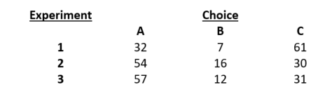
Note that the percentages across choices A – C are roughly the same for “sure-thing” Experiments 2 and 3. But the percentages deviate quite considerably from those for “unsure-thing” Experiment 1. Thus, Tversky and Shafir claim that their groups of Homo sapiens violate the Sure-Thing Principle.

Study Questions

1. Can you design a laboratory experiment to test the axiom that was not considered in this chapter—the Independence Axiom?
2. In Testing the Invariance and Dominance Axioms (Version 1), it is clear that broad framing leads to better outcomes than narrow framing. Can you think of a situation in real life where narrow framing could lead to a better outcome than broad framing?
3. Which biases discussed in Chapter 2 are most likely to be avoided through broad framing? Explain.
4. Can you think of three deficiencies associated with the laboratory experiments (discussed in this chapter) that were conducted with the researchers’ own students?
5. State in words why a violation of the Transitivity Axiom introduced in Chapter 3 also implies what we are calling a “preference reversal” in this chapter (e.g., see Testing the Invariance Axiom (Version 3)).
6. Can you design a simpler experiment to test for the Sure-Thing Principle than the one presented in this chapter?