Cable Properties of Neurons

Many schoolchildren in the United States are familiar with the completion of the Transcontinental Railroad in 1869 and how it transformed US history. Fewer are familiar with an event that happened about the same time: the successful deployment of a transatlantic telegraph cable between the United States and United Kingdom in 1866.

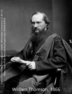
The Scottish scientist William Thomson was one of the greatest scientists of the 19th century. Along with Michael Faraday, whose work we met when we discussed the Nernst (Equilibrium) potential and the incorporation of the Faraday constant, Thomson made many key discoveries in thermodynamics, electricity, and magnetism. Among the most important, and yet least-known, of his works was making a 3000 km-long undersea telegraph cable feasible.

Several technological problems confronted the scientists and engineers who tried to lay the first transatlantic cable. Unlike telegraph cables that were surrounded by insulating air, undersea cables were surrounded by an electrically conductive medium (sea water) and this presented several technical problems. (Most of these are irrelevant for right now, but are detailed in this article.)

We have already seen the theoretical basis for one of Thomson’s greatest achievements: the telegraph cable equivalent of the node of Ranvier. Remember that even the best insulator has some leakage. This leakage, combined with a physical property called impedence, means that the electrical signal traveling down an axon gets smaller and smaller as it travels along the axon. The nervous system solves this problem by occasionally removing the myelin sheath at the node of Ranvier, where voltage-gated sodium and potassium channels “boost” the now-barely-above-threshold signal into a new action potential.

Thomson’s equivalent of the node of Ranvier was an instrument called the mirror galvanometer, which boosted a small telegraph signal periodically so that telegraph cable operators could avoid using huge voltages which would burn out the cable. For this achievement, and his other work on the transatlantic cable, Queen Victoria knighted Thomson in 1866. His record of achievement continued, and by the end of his life was so great he was made the first British scientist to join the House of Lords, in 1892.

Now we know him as Lord Kelvin, and the absolute temperature scale is named after him. Temperatures in Kelvin have the same increment as the Celsius scale, but the zero is set to absolute zero instead of the freezing point of water. (–273°C = 0 K; human body temperature of 37°C = 310 K, which was the number we used in deriving the Nernst equation.)

Much of the physics involved in deploying and operating the undersea telegraph cable applies to neurons as well. One has a cable (the cytoplasm of the axon, called the axoplasm for short); an insulating sheath (gutta-percha for the transatlantic cable, myelin for the axon); the cable/axon is surrounded by a conductive medium (seawater or extracellular fluid); and an electric current is traveling in one direction along the cable/axon. We therefore refer to these as cable properties of the neuron. They also apply to dendrites and unmyelinated axons, with some modifications.

We will only touch on the very superficial details of cable theory in neurons, but the interested student who is not afraid of some seriously tough mathematics is directed to the book I used in graduate school: Jack JJB, Noble D, and Tsien RW, Electric Current Flow in Excitable Cells (1975), which is now available for free.

For our purposes, we only need to master two concepts. The first is the easier one: as an electric current travels in space, it gets smaller in a steady and mathematically predictable way. Neuroscientists say it decrements in space.

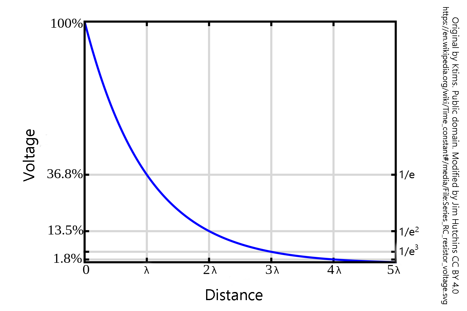
Let’s say lightning strikes a large lake where you are swimming. At a short distance from the place where the lightning strikes, you would be subjected to 300 million volts. Some distance away — for us, the distance doesn’t matter too much but the concept does — it would be at 110 million volts, or 36.8% of the original voltage. Twice that distance, and it would be at 40 million volts (13.5%); three times that distance, 15 million volts (5%); four times that distance, 5.4 million volts (1.8%), and five times that distance, 2 million volts (0.7%). To describe the mathematics, we use a constant you may have not seen before called e (Euler’s constant). It came up when we were discussing the Nernst equation, because it is the base used for the logarithm of the relative concentration (log_e), but we tossed it out pretty quickly in favor of the log₁₀ that is easier for most students to understand (but by no means easy, just easier). Like the more familiar π, e is an irrational, transcendental number (its digits go on forever).

To simplify things somewhat, there is a graph above that shows this concept. The distance over which the voltage decrements by 1/e (1/2.71828···) is called the length constant and symbolized by the Greek letter lambda (λ). At two length constants, the voltage is now the original voltage divided by e²; at three length constants, the original voltage divided by e³; and so forth. In our original example, after 20 length constants, the voltage of 300 million volts is divided by e²⁰ or a manageable 0.6 V, less than a AA battery.

For neurons, the length constant varies from about 1 mm in large-caliber axons to about 0.1 mm in smaller axons. For example, an action potential is about 100 mV. In the largest axons in the human body, that voltage will decrement to 1.8 mV (100/e⁴ mV) just 4 mm away from the axon hillock where we initiated the action potential. This is well below threshold for firing a new action potential. Without some sort of periodic boost like that provided by the node of Ranvier, there would not be much voltage left even a short distance away from the cell body of a neuron. Another strategy would be continuous conduction of an action potential, but as we’ve seen, that has the disadvantage of slowing down action potential conduction because of the time taken to open and close voltage-gated Na⁺ and K⁺ channels.

Notably, in dendrites, a very small voltage change at the synapse (typically less that 1 mV) becomes very small indeed over a distance of several millimeters.

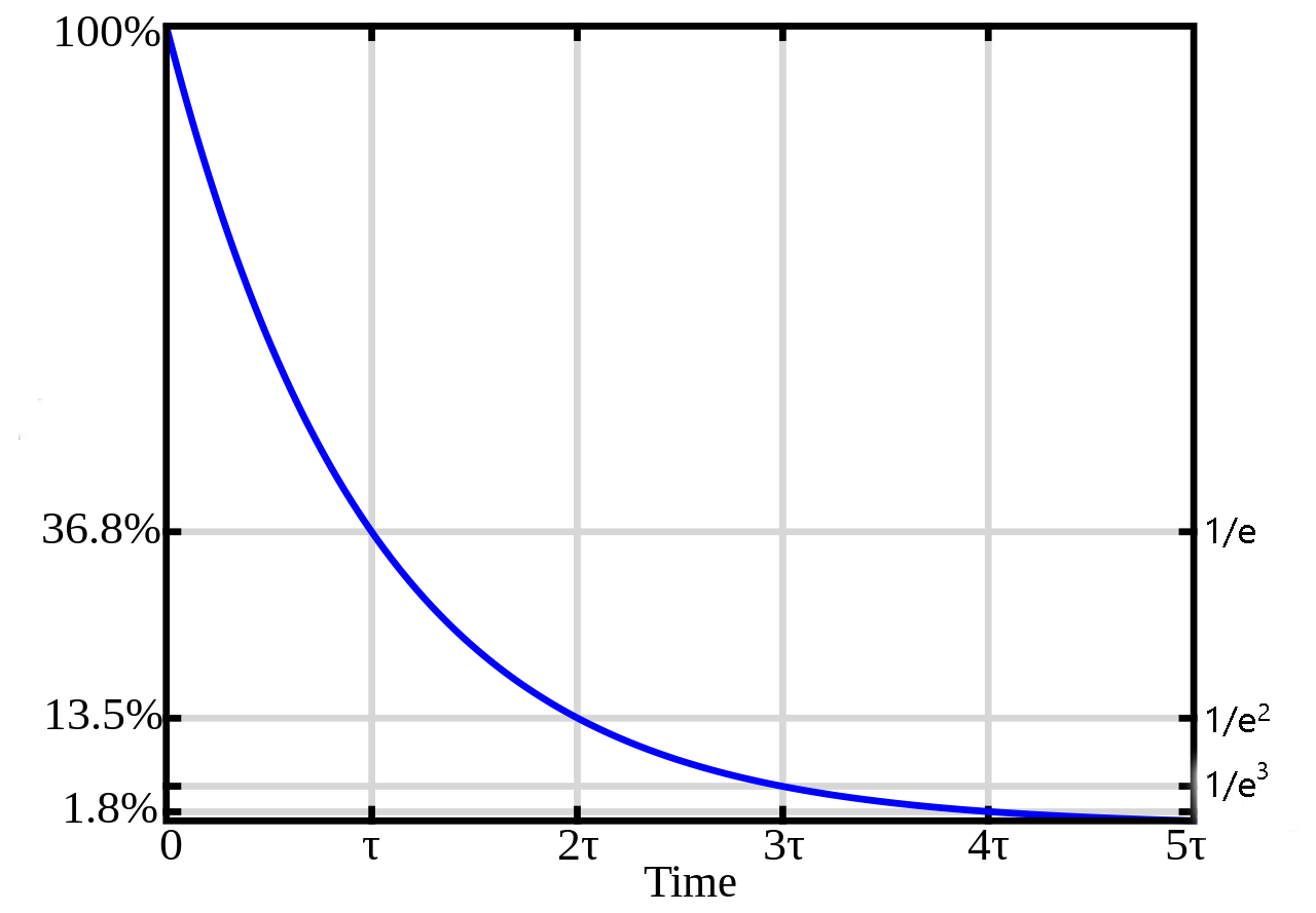
Now apply the same sort of analysis to time. Let’s say you’re wading in your favorite lake and lightning strikes in your exact location. You’re going to experience 300 million volts. But over a few seconds, that voltage change will have decremented and become near-zero fairly quickly. If you’re swimming in the exact spot where lightning struck yesterday, it is extremely unlikely that you will experience any change in voltage. Again, we describe a constant, now called the time constant (τ). Over time τ msec, the voltage in a neuron will decrease by 1/e.

In very general terms, τ is usually about 10-100 msec. Taking the larger of those, a 100 mV change in membrane potential will decrease to 37 mV just 0.1 sec later and to 14 mV just 0.2 sec later. Voltage changes in neurons don’t hang around for very long.

What seems like a bug in neurons will be a feature, as we will see: this drop in voltage over distance and time is used to process information, especially in dendrites and cell bodies. The placement and timing of synaptic inputs to a neuron is critical for information processing.