Data Analysis
This chapter will explore how we analyze the data we collect so that the researcher can make interpretations about the data.
Content:
- Introduction to Research Data Analysis
- Descriptive Statistics: Summarizing Data
- Inferential Statistics: Drawing Conclusions from Data
- Ensuring Accuracy and Validity in Data Analysis
- Peer Review and Replication: The Final Steps to Validity
- Ethical Considerations in Data Analysis
- Applying Data Analysis to Evidence-Based Practice
Objectives:
- Describe the purpose and significance of data analysis in nursing research and evidence-based practice.
- Differentiate between descriptive and inferential statistics and their roles in analyzing research data.
- Identify common statistical measures used in nursing research, including measures of central tendency and variability.
- Explain key inferential statistical tests, such as t-tests, chi-square tests, ANOVA, and regression analysis, and their applications in nursing studies.
- Interpret data presented in tables, charts, and graphs commonly found in nursing research articles.
- Discuss strategies for ensuring the accuracy and reliability of data analysis in quantitative research.
- Recognize common errors and biases in data analysis and their impact on research findings.
- Evaluate the statistical findings of a nursing research study and assess their implications for clinical practice.
- Explain the ethical considerations involved in research data analysis, including data integrity and responsible reporting of results.
- Apply knowledge of research data analysis to critically appraise nursing research articles and integrate findings into evidence-based practice.
Key Terms:
Analysis of Variance (ANOVA): A statistical method used to compare the means of three or more groups to see if at least one of the groups significantly differs from the others.
Central Tendency: A statistical measure that identifies a single value as a representative of a data set, commonly measured by the mean, median, and mode.
Chi-Square Test (χ² Test): A statistical test used to determine whether there is a significant association between categorical variables, often used for contingency tables.
Confidence Interval (CI): A range of values, derived from the sample data, that is used to estimate the true population parameter with a given level of confidence (usually 95%).
Data Analysis: The process of systematically applying statistical and logical techniques to describe, summarize, and evaluate data in research.
Descriptive Statistics: A set of statistical techniques used to summarize and organize data into meaningful patterns, typically through measures like mean, median, mode, Effect Size: A quantitative measure of the strength of a phenomenon or the size of the difference between groups, providing context to the statistical significance of a result.
and standard deviation.
Inferential Statistics: A branch of statistics that makes inferences and predictions about a population based on a sample of data, using techniques such as hypothesis testing and confidence intervals.
Mean (Arithmetic Mean): The average of a set of values, calculated by adding all the values and dividing by the number of values.
Median: The middle value in a data set when arranged in ascending or descending order, dividing the set into two equal halves.
Mode: The most frequently occurring value in a data set.
P-value: A statistical measure that helps determine whether the results of an experiment are statistically significant; it represents the probability of obtaining the observed results by chance. A p-value less than 0.05 is commonly considered statistically significant.
Regression Analysis: A statistical technique used to examine the relationship between one dependent variable and one or more independent variables, often to predict outcomes.
Reliability: Refers to the consistency and repeatability of a measurement.
Validity: Refers to the accuracy of a measurement in capturing what it is intended to measure.
Sampling Error: The difference between the sample statistic and the true population parameter, which can arise due to random variation in the sample selection.
Standard Deviation (SD): A measure of the dispersion or spread of data points around the mean; a high SD indicates greater variability in the data.
Statistical Significance: A determination of whether the observed result in a study is likely due to something other than random chance, often determined using p-values.
T-test: A statistical test used to compare the means of two groups to determine if there is a statistically significant difference between them.
Type I Error: A statistical error that occurs when a null hypothesis is incorrectly rejected (false positive).
Type II Error: A statistical error that occurs when a null hypothesis is incorrectly accepted (false negative).
Variability: A measure of how spread out or dispersed the values in a data set are, often quantified by the range, variance, and standard deviation.
Introduction
Evidence-based nursing practice relies on the accurate interpretation of research findings to guide clinical decision-making and improve patient outcomes. However, raw data alone do not provide meaningful insights until they are systematically analyzed. Research data analysis is the process of organizing, summarizing, and interpreting data to identify patterns, relationships, and trends that inform nursing practice.
In this chapter, we will explore the essential concepts of data analysis in nursing research, including statistical methods used to summarize and test research findings. Understanding descriptive and inferential statistics will equip nursing students with the skills to read and interpret research articles critically, evaluate the strength of evidence, and apply findings to patient care. Additionally, we will discuss ethical considerations related to data analysis, highlighting the importance of accuracy, transparency, and responsible reporting.
By mastering these concepts, nursing students will develop the foundational knowledge needed to engage with evidence-based practice, ensuring their clinical decisions are backed by rigorous research and sound statistical reasoning.
Defining Data Analysis
Research data analysis is the systematic process of examining, organizing, interpreting, and presenting data to uncover patterns, relationships, and insights. In nursing research, data analysis plays a crucial role in transforming raw information into meaningful conclusions that can guide clinical practice and evidence-based decision-making.
Data analysis allows researchers to:
- Summarize and describe collected data effectively.
- Identify trends and patterns that may impact nursing interventions.
- Test hypotheses and determine the significance of research findings.
- Draw conclusions that contribute to the advancement of nursing knowledge and patient care.
As we have learned previously, evidence-based practice (EBP) in nursing relies on the integration of best available research evidence, clinical expertise, and patient preferences to make informed care decisions. Research studies contribute to this body of knowledge, but without appropriate data analysis, their results cannot be trusted or applied to patient care.
Consider a study investigating whether a new pain management intervention is more effective than the current standard treatment. If the researchers fail to apply proper statistical tests or misinterpret their findings, nurses may be misled into adopting an ineffective or even harmful practice.
Key benefits of data analysis in EBP include:
✅ Identifying Best Practices: By analyzing patient outcomes, nursing researchers can determine which interventions are most effective.
✅ Improving Patient Outcomes: Proper data interpretation ensures that healthcare providers make data-driven decisions that enhance patient safety and well-being.
✅ Supporting Policy Changes: Well-analyzed research findings can guide hospital policies and healthcare regulations.
Nursing research involves both quantitative and qualitative data analysis, each serving different purposes:
- Quantitative Data Analysis: Focuses on numerical data, using statistical tools to measure relationships, compare variables, and test hypotheses.
- Qualitative Data Analysis: Involves interpreting non-numerical data (e.g., interviews, observations) to explore themes, experiences, and meanings.
While this chapter focuses on quantitative data analysis, it is essential to recognize that both types contribute to a comprehensive understanding of nursing research.
Foundational Assumptions of Data Analysis
Data analysis in research is built upon several foundational assumptions that ensure the validity, reliability, and meaningful interpretation of results. These assumptions guide researchers in selecting appropriate statistical methods and help prevent errors that could compromise the integrity of findings. Below are some key assumptions that underpin quantitative data analysis in nursing research. These include: 1) Data must be accurate and representative; 2) Data follow a certain level of measurement; 3) Data must be normally distributed; 4) Variables should be independent; 5) The relationship between variables should be linear; 6) There should be homogeneity of variance; and, 7) Statistical tests assume random sampling.
1. Data Must Be Accurate and Representative
For research findings to be valid, the data collected must accurately reflect the population being studied. This means:
-
- The sample should be representative of the larger population to avoid biases.
- Data collection methods must be systematic and standardized to ensure consistency.
- Researchers must minimize errors and missing data, as these can distort results.
🔹Example: If a study aims to evaluate patient satisfaction in a hospital, but only surveys young adult patients while ignoring older adults, the findings will not accurately represent the entire patient population.
2. Data Follow a Certain Level of Measurement
Research data can be categorized into four levels of measurement (nominal, ordinal, interval, and ratio), which determine the types of statistical analyses that can be performed:
Four Levels of Measurement:
Nominal: Categories without a numerical ranking (e.g., blood type, gender).
Key Features:
✅ Categories are mutually exclusive (each data point fits into only one).
✅ No numerical value or ranking is associated with the categories.
✅ Only counts and percentages can be used to describe nominal data.
🔹 Example in Nursing Research:
-
-
- Blood Type: A, B, AB, O
- Type of Hospital Unit: ICU, ER, Pediatrics, Surgery
- Wound Type: Pressure ulcer, burn, surgical wound
-
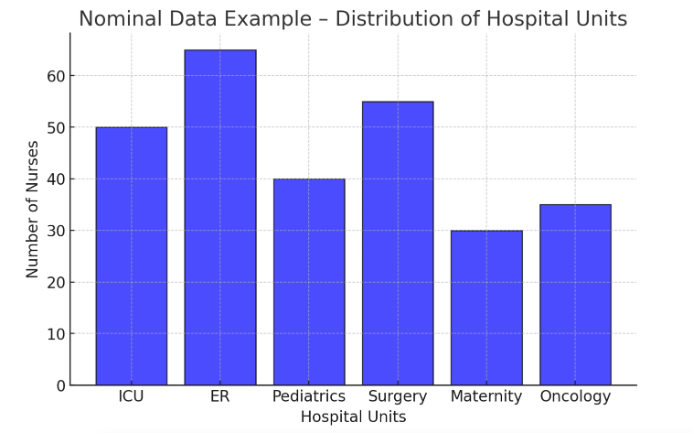
Figure Above: Nominal Data Example – Distribution of Hospital Units (A bar graph showing the number of nurses working in different hospital units.)
Ordinal: Categories with a meaningful order but unequal spacing (e.g., pain scales).
Key Features:
✅ Ordered categories but no precise spacing between ranks.
✅ Can use medians and percentile-based statistics (but not means).
✅ Often used in surveys, patient assessments, and pain scales.
🔹 Example in Nursing Research:
-
-
- Pain Scale: 1 = No Pain, 2 = Mild, 3 = Moderate, 4 = Severe, 5 = Worst Pain
- Patient Satisfaction Survey: Poor, Fair, Good, Excellent
- Glasgow Coma Scale: 3 (Comatose) to 15 (Fully Awake)
-
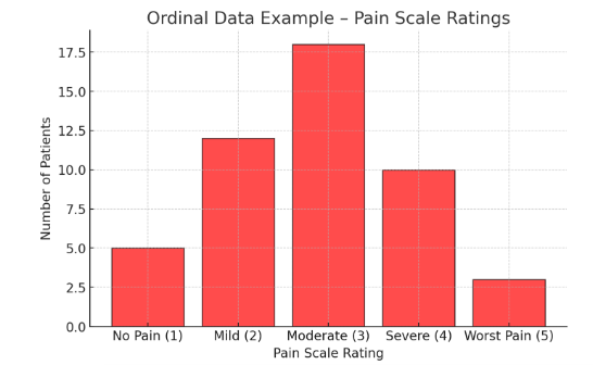
Figure Above: Ordinal Data Example – Pain Scale Ratings (A bar graph showing the distribution of patient pain scores on a 1-5 scale.)
Interval: Numeric data with equal spacing but no true zero (e.g., temperature in Celsius).
Key Features:
✅ Equal spacing between values (e.g., 10°F to 20°F is the same difference as 30°F to 40°F).
✅ Can calculate means, standard deviations, and perform statistical tests.
✅ No true zero (e.g., 0°F is not the absence of temperature).
🔹 Example in Nursing Research:
-
-
- Temperature in Celsius or Fahrenheit: 37°F, 98.6°F, 102°F
- SAT Scores: 500, 600, 700
- Patient Anxiety Score (on a scale of -10 to +10): -5, 0, 5
-
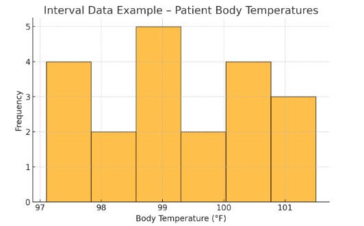
Figure Above: Interval Data Example – Patient Body Temperatures (A histogram displaying the distribution of patient temperatures in Fahrenheit.)
Ratio: Numeric data with equal spacing and a true zero (e.g., weight, blood pressure).
Key Features:
✅ All mathematical operations are possible (addition, subtraction, multiplication, division).
✅ A true zero point exists (e.g., 0 mg of medication means “no medication”).
✅ Most biomedical measurements fall into this category.
🔹 Example in Nursing Research:
-
-
- Heart Rate (bpm): 0 bpm (no heartbeat) to 120 bpm
- Patient Weight (kg): 0 kg (no weight) to 90 kg
- Medication Dosage (mg): 0 mg, 10 mg, 50 mg
-
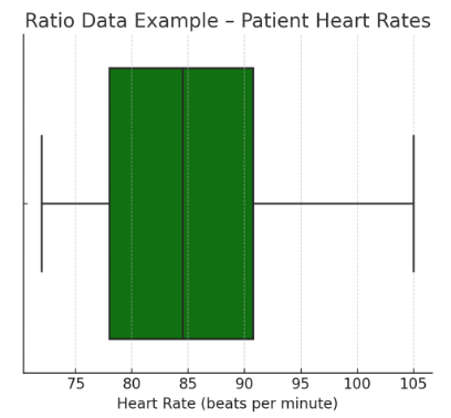
Figure Above: Ratio Data Example – Patient Heart Rates (A box plot displaying the range of patient heart rates with a true zero.)
Each type of data requires different statistical techniques. Using the wrong statistical test for a given level of measurement can lead to incorrect conclusions.
🔹 Example: A researcher should not calculate an average for “pain level” if it is measured using a categorical scale (e.g., “mild,” “moderate,” “severe”). Instead, they should use ordinal statistics such as medians or rankings.
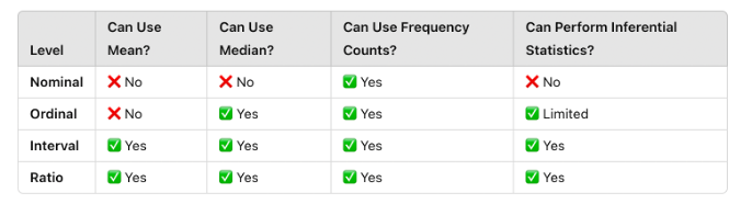
Figure Above: Comparison of Levels of Measurement
3. Data Must Be Normally Distributed (for Certain Tests)
Many statistical tests, such as t-tests and ANOVA, assume that data follow a normal distribution (bell-shaped curve). A normal distribution means:
- Most values cluster around the mean.
- The data is symmetrically distributed, with few extreme values.
Here is a standard deviation bell curve (normal distribution) showing the mean (μ) and standard deviations (±1 SD, ±2 SD, ±3 SD).
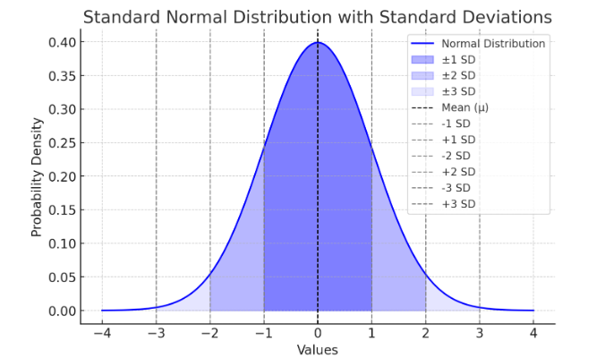
Figure Above: Normal Distribution. Notice that the “tails” on both sides of center (the mean) is symmetric (or close to it).
If data are not normally distributed, researchers may need to:
✅ Use non-parametric statistical tests (e.g., Mann-Whitney U test).
✅ Apply data transformations (e.g., logarithmic transformation).
🔹 Example: If researchers measure hospital wait times and find that most patients wait 10-15 minutes, but a few wait over 2 hours, the data is skewed rather than normally distributed. This may require special statistical approaches.
Here is a positively skewed (right-skewed) distribution, where the mean (μ) is greater than the median due to the long tail on the right.
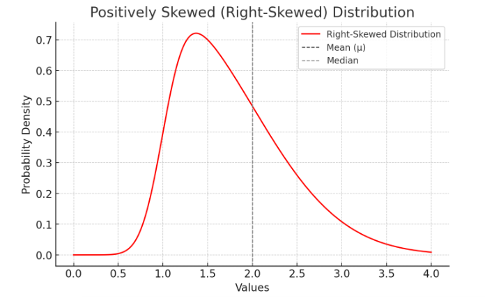
Figure Above: Skewed Distribution. Notice how one side of the mean is longer than the other side.
4. Variables Should Be Independent (for Many Tests)
Many statistical tests assume that observations are independent, meaning that one participant’s data does not influence another’s. If data points are dependent (e.g., repeated measures from the same individuals), specialized statistical approaches are required.
🔹 Example: A study measuring the effect of a new medication on blood pressure should ensure that patients are not sharing medications, as this could introduce dependence between samples.
5. The Relationship Between Variables Should Be Linear (for Correlation and Regression)
When analyzing relationships between variables (e.g., between exercise and heart rate), researchers often assume that the relationship is linear, meaning it forms a straight-line pattern on a graph. If the relationship is curvilinear or complex, standard linear tests (such as Pearson correlation) may be inappropriate.
🔹 Example: If a study examines the link between stress and performance, it may find a curved relationship (e.g., moderate stress improves performance, but excessive stress reduces it). In such cases, non-linear models are needed.
6. There Should Be Homogeneity of Variance (Equal Variability in Groups)
Many statistical tests assume that different groups being compared have similar variability (spread of scores). This is known as homogeneity of variance or homoscedasticity. If one group has much more variability than another, researchers must adjust their analyses.
🔹 Example: If a study compares pain relief in two groups—one receiving a placebo and another receiving strong pain medication—variability in pain scores may differ significantly between the groups, requiring adjustments like the Welch’s t-test.
7. Statistical Tests Assume Random Sampling
For statistical results to be generalizable, the sample must be randomly selected from the population. If sampling is biased or non-random, results may not accurately apply to broader populations.
🔹 Example: If a study on nurse burnout only surveys nurses from a single hospital, the findings may not reflect burnout levels in nurses across different healthcare settings.
Why These Assumptions Matter
Failing to meet these assumptions can lead to:
❌ Invalid conclusions – Misinterpretation of data can lead to false findings.
❌ Reduced reliability – Results may not be repeatable in future studies.
❌ Inaccurate clinical application – Misleading research could result in poor patient care decisions.
By understanding and upholding these foundational assumptions, nurses and researchers can ensure that data analysis is accurate, ethical, and applicable to real-world clinical settings.
Ethical Dilemma Example
A nursing researcher conducting a study on a new pain management intervention finds that the results are not statistically significant. Under pressure from hospital administrators and funding agencies, the researcher considers manipulating the data—removing outliers, using a less appropriate statistical test to achieve significance, or selectively including participants with favorable outcomes. This raises ethical concerns about integrity, transparency, and the potential harm of misleading findings in evidence-based practice. Should the researcher alter the data to support the intervention, or uphold ethical standards by reporting the true results?
Descriptive Statistics
Descriptive statistics are used to summarize and organize raw data to make it easier to interpret. In essence, it simply is telling us more about our data by organizing it before further analysis is done. In nursing research, these statistics help researchers describe trends, distributions, and variations within a dataset without making conclusions beyond the data collected. Meaning, descriptive statistics do not answer the hypothesis nor draw inferences about generalizability of our outcome.
Descriptive statistics fall into three main categories:
- Measures of Central Tendency – Identify the center of a data set (mean, median, mode).
- Measures of Variability (Dispersion) – Show the spread of data (range, standard deviation, variance).
- Data Visualization Techniques – Represent data using charts, graphs, and tables for easier interpretation.
Measures of Central Tendency
1. Mean (Average)
The mean is the sum of all values divided by the number of observations. It is useful for normally distributed data but can be affected by outliers (extreme values).
🔹 Example: A study measures the number of hours nurses spend documenting patient records per shift:
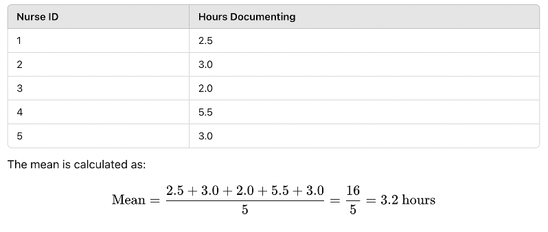
Figure Above: Calculation of the Mean
2. Median (Middle Value)
The median is the middle value when data are arranged in ascending order. It is useful for skewed distributions because it is not affected by outliers.
🔹 Example: Using the same nurse documentation data:
Sorted data: 2.0, 2.5, 3.0, 3.0, 5.5
The median is 3.0 hours (middle value).
3. Mode (Most Frequent Value)
The mode is the most frequently occurring value in a dataset. It is useful for categorical data where the most common category is important.
🔹 Example: A study tracks the most common type of wound care dressing used in a hospital:
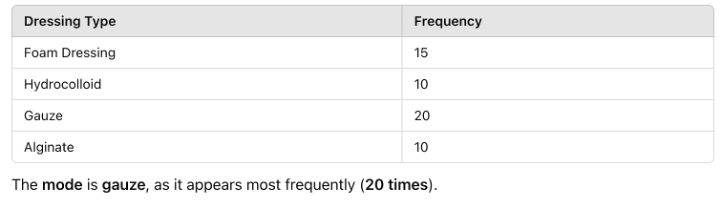
Figure Above: Calculation of Mode
Measures of Variability (Dispersion)
The measures of variability show the spread of data (range, standard deviation, variance).
1. Range (Difference Between Highest & Lowest Values)
The range shows the spread of data by subtracting the lowest value from the highest value.
🔹 Example: In the nurse documentation time dataset:
Highest value: 5.5 hours
Lowest value: 2.0 hours
Range = 5.0 – 2.0 = 3.5 hours
2. Standard Deviation (SD) (Average Distance from the Mean)
The standard deviation indicates how spread out the data points are around the mean.
A low SD means the data points are close to the mean, while a high SD means they are more spread out. All data should normally fall within 68% of 1 SD, and 95% of data within 2 SDs. See Figure 9.11.
🔹 Example: If two hospital units measure patient wait times, one with low SD has consistent wait times, while another with high SD has highly variable wait times.
Here’s a visual representation of standard deviation:

Figure Above: Standard Normal Distribution with Standard Deviations
Ponder This
Imagine you are reviewing a research study on fall prevention strategies in elderly patients. The study presents only raw data (e.g., fall occurrences per month). How would descriptive statistics, such as mean, standard deviation, and graphs, help you interpret the results and determine the effectiveness of the intervention?
Data Visualization – Making Sense of Data
Graphs and charts are essential for quickly interpreting research data. Here are common visualization methods:
1. Frequency Distribution Table
A frequency distribution shows how often each value appears in a dataset.
🔹 Example: Patient pain levels rated on a scale from 1 to 5:
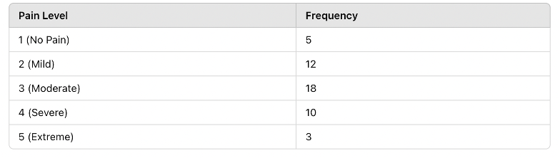
Figure Above: Frequency Distribution Table – This table summarizes how pain scores are distributed in the sample population.
2. Histogram (Bar Graph for Numerical Data)
A histogram shows the frequency of values in a dataset. Below is a histogram of patient heart rates recorded in a study:
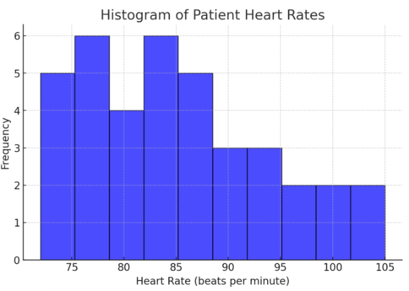
Figure Above: Histogram of Patient Heart Rates (Graph displaying heart rate data distribution, with most patients clustered around normal heart rate ranges.)
3. Box Plot (Shows Variability & Outliers)
A box plot (or box-and-whisker plot) represents medians, quartiles, and outliers in a dataset. It is useful for identifying skewness and variability in data.
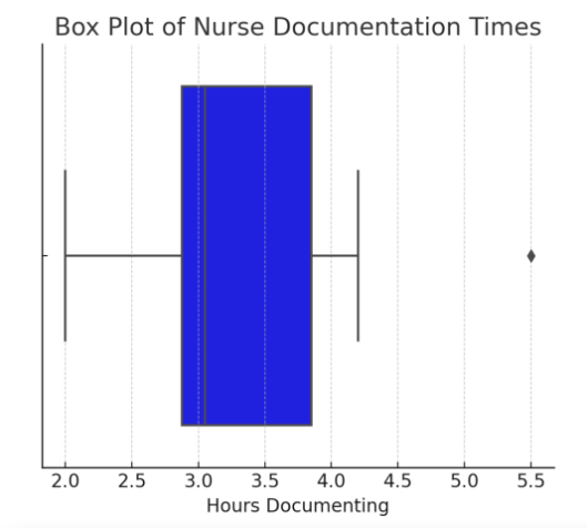
Figure Above: Box Plot of Nurse Documentation Times (Box plot displaying median time spent on documentation, with an outlier visible.)
![]() Hot Tip! When analyzing data, always check for outliers before calculating the mean—a single extreme value can skew your results and give a misleading summary of the data!
Hot Tip! When analyzing data, always check for outliers before calculating the mean—a single extreme value can skew your results and give a misleading summary of the data!
Inferential Statistics: Drawing Conclusions from Data
While descriptive statistics help summarize and organize data, they do not allow researchers to draw conclusions beyond the dataset. Inferential statistics, on the other hand, allow researchers to make predictions and generalizations about a population based on a smaller sample. These statistical methods are essential in nursing research, where studies often use a subset of patients, nurses, or healthcare settings to make broader conclusions about clinical practices, patient care, or healthcare outcomes.
For example, a hospital may conduct a study on 100 elderly patients to test whether a new fall prevention program reduces fall rates. Using inferential statistics, researchers can determine if the findings apply to all elderly patients, not just those in the study. Inferential statistics rely on probability theory, allowing researchers to assess whether results are statistically significant or merely due to chance.
In evidence-based practice (EBP), inferential statistics are crucial in evaluating whether an intervention is effective, determining differences between groups, identifying relationships between variables, and supporting data-driven decision-making in healthcare.
Inferential statistics answer questions like:
- Does a new pain management intervention significantly reduce pain compared to standard care?
- Is there a relationship between nurse staffing levels and patient fall rates?
- Can we predict infection rates based on hospital hygiene compliance?
Why Inferential Statistics Matter in Nursing Research
Inferential statistics allow nurses and healthcare professionals to:
✅ Determine if an intervention is effective (e.g., testing whether a new wound care treatment leads to faster healing).
✅ Compare groups and detect differences (e.g., evaluating whether ICU nurses experience higher stress levels than surgical nurses).
✅ Identify relationships between variables (e.g., analyzing whether increased nurse staffing levels reduce patient complications).
✅ Make data-driven decisions that improve patient care and policy development.
Unlike descriptive statistics, which describe only the data collected, inferential statistics use probability to estimate whether the results are applicable to a broader population. This is done through hypothesis testing, confidence intervals, and statistical significance testing.
From Sample to Population: How Inference Works
Because it is often impractical to study an entire population, researchers use samples—smaller, carefully selected groups that represent the population. Inferential statistics help determine whether findings from a sample can be generalized to the whole population.
For example, if a study finds that 40 ICU patients experienced a significant reduction in pain after a new treatment, inferential statistics help researchers determine whether the same effect would likely be observed in all ICU patients, not just those in the study.
Key Concepts in Inferential Statistics:
🔹 Hypothesis Testing – Determines whether observed effects are real or due to chance.
🔹 P-Values & Confidence Intervals – Measures statistical significance and certainty.
🔹 Comparing Groups (t-Tests, ANOVA) – Determines if differences between groups are meaningful.
🔹 Examining Relationships (Chi-Square, Regression Analysis) – Identifies associations and predictions between variables.
By understanding inferential statistics, nursing students and healthcare professionals can critically evaluate research, interpret findings, and apply evidence-based interventions that lead to better patient outcomes.
Key Concepts in Inferential Statistics
Population vs. Sample
In research, the population refers to the entire group of individuals a study aims to understand, such as all ICU nurses in a country. Since studying an entire population is often impractical, researchers select a sample, a smaller group intended to represent the larger population. Generalizability refers to how well the findings from the sample can be applied to the population.
For instance, if researchers study nurse burnout by surveying 200 nurses from different hospitals, they use inferential statistics to determine whether their results represent all nurses rather than just those in the study. The accuracy of this generalization depends on sampling methods, sample size, and statistical techniques used in the study.
Probability and Statistical Significance (p-values & Confidence Intervals)
Inferential statistics rely on probability to assess the likelihood that research findings are meaningful. One of the most important concepts in inferential statistics is the p-value, which measures how likely the observed results occurred by chance. A p-value less (<) than 0.05 is commonly considered statistically significant, meaning there is less than a 5% probability that the results happened randomly.
For example, a study on hand hygiene compliance finds that improved handwashing techniques reduce infection rates, with a p-value of 0.03. Since 0.03 < 0.05, researchers conclude that the handwashing intervention likely has a real impact on reducing infections.
Another critical concept is the confidence interval (CI), which provides a range of values within which the true population parameter is likely to fall. A 95% confidence interval means researchers are 95% confident that the true effect lies within a given range.
🔹 Example: A study finds that a new IV insertion technique reduces infection rates with a 95% confidence interval of 2% to 8%. This means the true reduction in infections is likely between 2% and 8%, rather than just a single percentage.
Here is an example of a 95% Confidence Interval, illustrating the sample mean (blue dashed line) and the confidence interval range (shaded red area between lower and upper bounds).

Figure Above: Confidence Interval
Common Inferential Statistics
Researchers use different inferential statistical tests depending on the study design and type of data being analyzed. Below are some of the most frequently used tests in nursing research.
Comparing Two Groups: t-Test
A t-test determines whether there is a significant difference between the means of two groups. This test is commonly used in nursing research to compare patient outcomes, staff performance, or treatment effectiveness.
🔹 Example: A study compares nurses’ stress levels in two hospital units:
- Unit A (low staffing): Mean stress score = 8.2
- Unit B (adequate staffing): Mean stress score = 6.5
- p-value = 0.01 → Since 0.01 < 0.05, the difference is statistically significant, indicating that staffing levels affect nurse stress.
Here is a t-Test example – Nurse Stress Scores in Two Units, illustrating the higher stress levels in the low-staffed unit (Unit A) compared to the adequately staffed unit (Unit B).
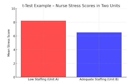
Figure Above: t-Test Example – Nurse Stress Scores in Two Units (A bar graph comparing mean stress scores, showing higher stress in low-staffed units.)
Comparing Categorical Data: Chi-Square Test
A chi-square test examines relationships between categorical variables to determine if differences are statistically significant.
🔹 Example: A study investigates whether infection rates differ between nurses who follow strict hand hygiene and those who do not.
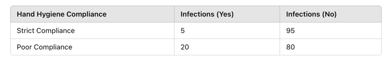
Figure Above: Chi-Square Test Example – Infection Rates by Hand Hygiene Compliance (Bar graph showing higher infection rates in nurses with poor hand hygiene compliance.)
- Chi-square test result: p = 0.02
- Since 0.02 < 0.05, the results suggest a significant relationship between hand hygiene and infection rates.
Comparing More Than Two Groups: ANOVA (Analysis of Variance)
ANOVA is used when comparing three or more group means to determine if there are statistically significant differences.
🔹 Example: A study examines nurse burnout levels across different shifts:
-
- Day Shift: Mean burnout score = 5.6
- Evening Shift: Mean burnout score = 6.8
- Night Shift: Mean burnout score = 7.5
- p-value = 0.04 → Since 0.04 < 0.05, the results indicate that shift timing significantly affects burnout levels.
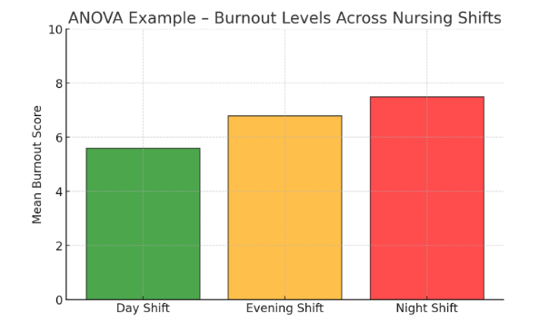
Figure Above: ANOVA Example – Burnout Levels Across Nursing Shifts (Bar graph showing highest burnout scores in night shifts.)
Examining Relationships Between Variables: Regression Analysis
Regression analysis identifies how one variable influences another and helps predict outcomes.
🔹 Example: A study investigates whether increased patient load predicts higher nurse burnout.
-
- Independent variable (X): Number of patients per nurse
- Dependent variable (Y): Burnout score
- Regression coefficient: +0.45 → Each additional patient increases burnout scores by 0.45 points.
In the example below, this is a scatterplot with a positive correlation between patient load and nurse burnout. The regression line (in red) highlights the trend that as patient load increases, burnout scores tend to rise.
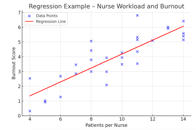
Figure Above: Regression Example – Nurse Workload and Burnout (Scatterplot showing a positive correlation between patient load and burnout.)
Why Inferential Statistics Matter in Nursing Research
Inferential statistics help translate research into practice by allowing healthcare professionals to determine if interventions are effective (e.g., testing whether a new fall prevention strategy reduces patient falls). It also allows for comparison of different treatment approaches (e.g., assessing whether one pain management technique is superior).
It also assists in identifying factors influencing patient care (e.g., analyzing how nurse-patient ratios impact patient safety). It supports policy changes (e.g., using research findings to advocate for better staffing levels in hospitals). By understanding inferential statistics, nursing students, educators, and clinicians can critically appraise research findings and make data-driven decisions that improve patient care.
Ponder This
Imagine you are reviewing a study comparing patient fall rates before and after implementing a new fall prevention program.
The results show a 10% reduction in falls, but the p-value is 0.07 (greater than 0.05).
Should the intervention be adopted in hospitals? What additional statistical tests or evidence might be needed?
Ensuring Accuracy and Validity in Data Analysis
The reliability of nursing research depends on the accuracy and validity of data analysis. Without proper safeguards, errors in data collection, statistical interpretation, or reporting can lead to misleading conclusions, potentially impacting patient care and evidence-based practice. Ensuring data integrity requires careful planning, systematic data handling, and rigorous statistical analysis. In this section, we explore strategies for maintaining accuracy and validity, including methods to detect errors, biases, and inconsistencies in research data.
Accuracy vs. Validity: What’s the Difference?
In nursing research, accuracy and validity are two fundamental concepts that ensure data integrity and the reliability of study findings. Though they are closely related, they refer to different aspects of measurement and analysis. A study can be accurate but not valid, valid but not accurate, both, or neither. Understanding the distinction is crucial for evaluating research quality and applying findings to evidence-based practice.
Accuracy refers to how close a measured value is to the true or actual value. If data are accurate, they correctly represent the real-world phenomenon being studied. Validity refers to how well a study measures what it is intended to measure. Even if measurements are accurate, they must also be relevant to the research question to be considered valid.
Accuracy:
A nurse measures a patient’s blood pressure using an automated monitor. If the patient’s actual blood pressure is 120/80 mmHg, but the monitor consistently records 118/79 mmHg, the readings are very close to the true value—indicating high accuracy.
Common Threats to Accuracy:
🔹 Equipment Malfunctions: A faulty thermometer may consistently read temperatures 2°F lower than actual values.
🔹 Human Error: A nurse may incorrectly document a patient’s weight, leading to inaccurate data.
🔹 Environmental Factors: Noise or lighting conditions may affect the accuracy of hearing or vision tests.
Validity:
A researcher develops a new pain scale that asks patients how well they slept the previous night. While this may provide useful information, sleep quality is not a direct measure of pain, making the scale invalid for measuring pain levels.
Common Threats to Validity:
🔹 Using the Wrong Measurement Tool: A kitchen scale may accurately measure weight, but it is not valid for measuring blood pressure.
🔹 Poorly Designed Surveys: A patient satisfaction survey with leading questions may not truly reflect patient experiences.
🔹 Lack of Experimental Control: If a study on nurse burnout does not account for differences in shift length, workload, or staffing levels, its conclusions may not be valid.
A study or measurement can be:
- Accurate but not valid → The measurement is correct but not relevant to what is being studied.
- Valid but not accurate → The measurement is useful but contains errors or inconsistencies.
- Both accurate and valid → The best-case scenario, where data are both correct and meaningful.
For example, a thermometer may consistently measure 98.2°F (high accuracy), but if it is incorrectly calibrated and should read 97.8°F, it is not valid.
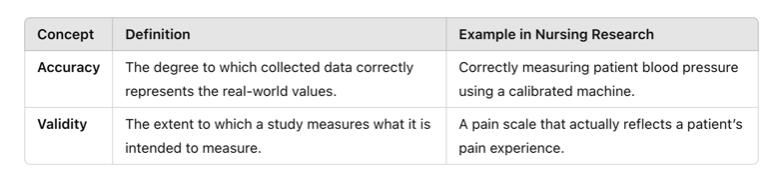
Figure Above: Accuracy and Validity
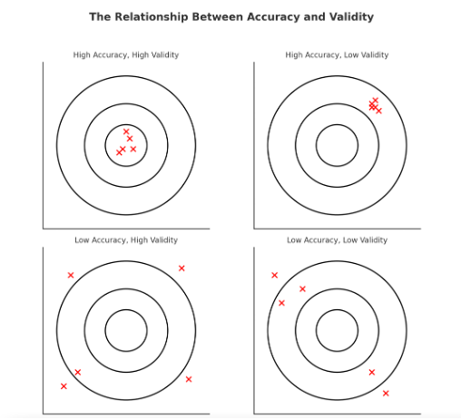
Figure Above: The Relationship Between Accuracy and Validity (Diagram illustrating that data can be accurate but not valid, valid but not accurate, both, or neither.)
Common Errors in Data Analysis
Even well-designed nursing studies can suffer from errors that compromise accuracy and validity. These errors typically fall into two categories:
1. Measurement Errors
These occur when data is not collected or recorded correctly, affecting accuracy.
🔹 Example: A nurse records patient weights but forgets to remove the weight of a heavy blanket, leading to inflated values.
2. Statistical Errors
These occur when researchers misapply statistical techniques or misinterpret findings.
🔹 Example: A researcher uses a t-test (for two groups) when analyzing a study with three or more groups, leading to incorrect conclusions.
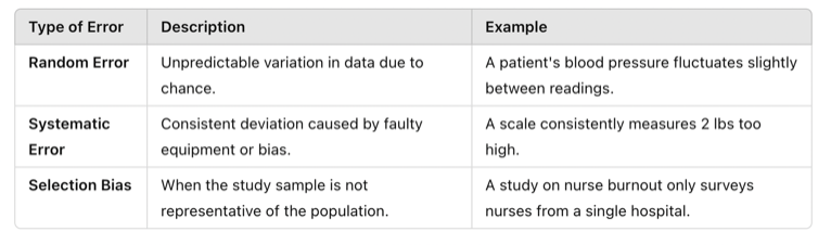
Table Above: Errors and Bias
Strategies to Improve Accuracy in Data Analysis
Use Reliable Measurement Tools
-
- Ensure equipment (e.g., BP cuffs, thermometers) is calibrated and tested before data collection.
- Standardize procedures to ensure consistent data collection across different researchers.
🔹 Example: If multiple nurses are recording patient pain levels, they should all use the same validated pain scale to reduce variability.
Double-Check and Clean Data
-
- Review datasets for outliers, missing values, and inconsistencies.
- Use software functions to detect duplicate entries or unusual patterns.
Ensuring Validity in Statistical Analysis
Statistical analysis is a powerful tool in nursing research, allowing researchers to examine relationships, compare groups, and make inferences about populations. However, the validity of statistical analysis determines whether these conclusions are meaningful and applicable to real-world practice. If the statistical methods used are flawed, even a well-designed study can produce misleading results. Ensuring validity in statistical analysis requires choosing appropriate statistical tests, controlling for confounding variables, and minimizing bias.
A critical step in ensuring validity is selecting the appropriate statistical test based on the type of data and research question. Using the wrong test can lead to incorrect conclusions and misinterpretation of findings.
For example, if a study examines whether a new wound care dressing leads to faster healing compared to a standard dressing, researchers need to compare the mean healing times between the two groups. A t-test, which compares the means of two independent groups, is appropriate. However, if the researcher mistakenly uses a chi-square test, which is designed for categorical data, the results would not be valid.
Using the correct statistical test ensures that results accurately reflect the underlying relationships within the data and are valid for interpretation in clinical practice. The following table summarizes which statistical tests should be used based on the research objective:
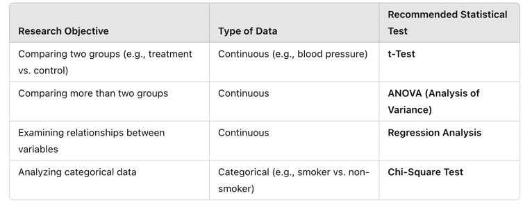
Table Above: Recommended Statistical Tests
Controlling for Confounding Variables
A major threat to the validity of statistical analysis is the presence of confounding variables—factors that may influence the relationship between the independent and dependent variables, leading to incorrect conclusions.
For example, a study finds that patients who exercise have lower cholesterol levels. However, if the study fails to account for diet, which also affects cholesterol, it may incorrectly attribute the difference solely to exercise.
To enhance validity, researchers can use statistical techniques such as:
- Stratification – Analyzing subgroups separately (e.g., comparing patients with similar dietary habits).
- Multivariate Regression Analysis – Adjusting for multiple confounders to isolate the true effect of the independent variable.
🔹 Example: A study examining the effect of nurse-to-patient ratios on patient outcomes should control for hospital size, patient severity, and staff experience to ensure the findings reflect the actual impact of nurse staffing levels. By identifying and adjusting for confounders, researchers can produce more valid and clinically relevant conclusions.
Even with a well-structured analysis, bias can distort results and threaten validity. Common sources of bias include:
- Selection Bias – When study participants are not representative of the target population.
- Confirmation Bias – When researchers focus only on data that supports their hypothesis, ignoring conflicting results.
- Publication Bias – When studies with statistically significant results are more likely to be published, while negative or neutral findings are overlooked.
Reducing Bias to Improve Validity
To mitigate these biases, researchers should:
✅ Use random sampling to ensure the study population represents the broader population.
✅ Conduct blinded studies, where researchers and participants do not know treatment assignments.
✅ Report all findings, including negative or non-significant results, to provide a complete picture.
🔹 Example: A study comparing pain relief between two medications should ensure that both patients and researchers are blinded to the treatment assignments. If participants know which medication they are receiving, their perceptions of pain relief may be influenced, introducing bias into the results.
Ensuring Statistical Significance and Clinical Relevance
Understanding p-Values and Confidence Intervals
Statistical results must be both statistically significant and clinically meaningful. The p-value is a key measure in statistical testing:
- A p-value < 0.05 suggests that results are statistically significant, meaning the observed effect is unlikely to be due to chance.
- A p-value > 0.05 indicates that the observed effect may have occurred by random variation and is not statistically significant.
However, statistical significance does not always mean a result is clinically important. A small, statistically significant difference may have little real-world impact.
🔹 Example: A study finds that a new antihypertensive medication reduces systolic blood pressure by 1 mmHg with a p-value of 0.01. While statistically significant, this small reduction may not be clinically meaningful for improving patient health.
Confidence intervals (CIs) provide additional insight by estimating the range within which the true effect likely falls. A narrow confidence interval indicates greater precision, while a wide confidence interval suggests more uncertainty in the estimate.
This following figure is of a 95% Confidence Interval, visually representing how confidence intervals help interpret statistical significance and precision. The plot includes:
- Sample Mean (blue dashed line) – The central estimated value.
- Lower and Upper Confidence Interval Bounds (red dashed lines) – The range in which the true population mean is likely to fall 95% of the time.
- Shaded Confidence Interval (red area) – Illustrating the spread of possible true values.
The following figure highlights how confidence intervals provide a margin of certainty around statistical estimates, helping researchers assess the reliability of findings.
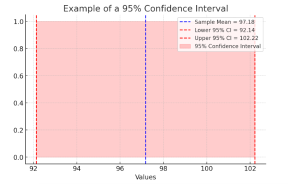
Figure Above: Example of a 95% Confidence Interval (A visual representation showing how confidence intervals help interpret statistical significance and precision.)
![]() Hot Tip! Always consider both statistical significance (p-value) and clinical relevance (effect size and confidence intervals) before applying research findings to practice!
Hot Tip! Always consider both statistical significance (p-value) and clinical relevance (effect size and confidence intervals) before applying research findings to practice!
Understanding Type I and Type II Errors in Data Analysis
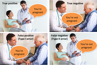
In data analysis, particularly in statistical hypothesis testing, making the right conclusion is crucial. However, errors are always a possibility when interpreting data. Two fundamental types of errors, Type I and Type II errors, can significantly impact decision-making in research, medicine, business, and various scientific disciplines. These errors arise from incorrect conclusions about the null hypothesis (H₀) and can lead to real-world consequences, from misdiagnosing a patient to approving ineffective medical treatments. Understanding these errors helps researchers make informed decisions about data collection, analysis, and interpretation, leading to more reliable and meaningful conclusions.
Type I Error
A Type I error occurs when a researcher incorrectly rejects the null hypothesis (H₀) when it is actually true. This is often called a “false positive” because the test falsely suggests an effect or relationship exists when it does not.
Example of Type I Error
Imagine a clinical trial for a new drug designed to lower blood pressure. The null hypothesis (H₀) states that the drug has no effect. If the study finds a significant effect and rejects H₀, but in reality, the drug is ineffective, then the study has committed a Type I error. This means the drug may be approved despite having no real benefit, leading to wasted resources and potential harm to patients.
Probability of Type I Error (Alpha, α):
The probability of making a Type I error is denoted by α (alpha), also known as the significance level. Common choices for α include:
- 0.05 (5%) – A 5% chance of incorrectly rejecting a true null hypothesis.
- 0.01 (1%) – A 1% chance of making a Type I error (stricter test).
Researchers choose α before conducting a test. A lower α reduces the chance of a Type I error but increases the risk of a Type II error (discussed below).
Consequences of Type I Error:
Approving an ineffective medical treatment.
- Wrongfully convicting an innocent person in court.
- Implementing unnecessary policies based on faulty data.
- Wasting resources on non-existent effects.
To minimize Type I errors, researchers use lower α levels, replicate studies, and apply multiple testing corrections (such as the Bonferroni correction).
Type II Error
A Type II error occurs when a researcher fails to reject the null hypothesis (H₀) when it is actually false. This is called a “false negative” because the test misses a real effect or relationship.
Example of Type II Error
Consider a COVID-19 diagnostic test. The null hypothesis (H₀) states that a patient does not have COVID-19. If the test incorrectly fails to detect an infection, a Type II error has occurred. The patient may be told they are healthy when, in reality, they are infected and could spread the disease to others.
Probability of Type II Error (Beta, β)
The probability of making a Type II error is represented by β (beta). The power of a statistical test (1 – β) is the probability of correctly detecting a true effect. A higher power reduces the likelihood of a Type II error.
Factors That Increase Type II Errors
- Small sample size (not enough data to detect real effects).
- High variability in data (noise can obscure patterns).
- Too strict of an alpha level (e.g., lowering α from 0.05 to 0.01 increases Type II errors).
- Weak effect size (small differences may not reach statistical significance).
Consequences of Type II Error
- Failing to detect a harmful side effect of a drug.
- Allowing a criminal to go free due to lack of evidence.
- Missing early signs of climate change in environmental research.
- Dismissing a valid scientific theory because of insufficient statistical power.
To minimize Type II errors, researchers increase sample sizes, choose appropriate α levels, and use power analysis to determine the number of observations needed for reliable results.
Balancing Type I and Type II Errors
Type I and Type II errors have an inverse relationship—reducing one increases the likelihood of the other. The challenge is to strike a balance based on context and the consequences of each error. In medicine, Type I errors (approving an ineffective drug) may be more dangerous than Type II errors (failing to detect an effective drug).
- In criminal justice, Type I errors (wrongful conviction) are often considered worse than Type II errors (letting a guilty person go free).
- In scientific research, balancing these errors depends on the risk of false discoveries vs. missing true findings.
Statisticians often adjust α and β depending on the stakes involved. In high-risk scenarios (e.g., medical trials, aerospace safety, forensic evidence), minimizing Type I errors is a priority. In exploratory research, reducing Type II errors to avoid missing new discoveries may be more important.
Real-World Applications of Type I and Type II Errors
- Medical Diagnostics – False positives (Type I) can lead to unnecessary treatments, while false negatives (Type II) may delay care for serious illnesses.
- Business and Marketing – Companies analyzing customer trends may mistakenly invest in ineffective strategies (Type I) or miss out on profitable opportunities (Type II).
- Scientific Research – A Type I error could falsely support an ineffective treatment, while a Type II error could cause researchers to overlook a life-saving drug.
- Machine Learning and AI – An AI model predicting fraud could wrongly flag innocent customers (Type I) or fail to detect actual fraud (Type II), affecting business decisions.
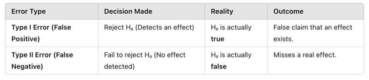
Figure Above: Balancing Type I and Type II Errors
Strategies to Minimize Errors in Data Analysis
Adjust α levels wisely (stricter α for high-risk studies, more relaxed α for exploratory research).
- Increase sample size to improve statistical power and reduce Type II errors.
- Use replication studies to confirm findings and reduce Type I errors.
- Perform power analysis to ensure sufficient data is collected.
- Apply corrections for multiple comparisons to avoid false positives in large datasets.
To reduce the likelihood of these errors, researchers carefully select appropriate statistical tests based on their data type and research question. Below are common statistical tests and how they relate to Type I and Type II errors.
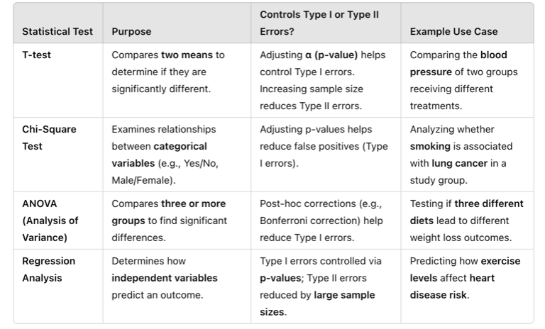
Table Above: Statistical Tests to Manage Type I and Type II Errors
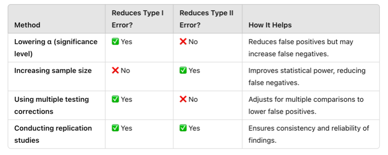
Table Above: Strategies to Minimize Type I and Type II Errors
Practical Application: Type I Error in Medical Diagnosis
A new cancer screening test claims to detect early-stage breast cancer. Researchers set the significance level (α) at 0.05 to balance the risk of false positives.
Outcome:
- The test incorrectly identifies 5% of healthy patients as having cancer (Type I error).
- These patients undergo unnecessary biopsies, psychological distress, and costly follow-up tests.
Prevention Strategies:
-
- Lower α to 0.01 for stricter testing.
- Perform multiple screening tests before confirming a diagnosis.
Practical Application: Type II Error in Drug Effectiveness
A pharmaceutical company tests a new drug for lowering blood pressure. The sample size is too small, and the statistical power is low.
Outcome:
- The study fails to detect the drug’s effectiveness, even though it actually works (Type II error).
- The drug is not approved, and a potentially life-saving treatment is dismissed.
Prevention Strategies:
- Increase sample size to boost statistical power.
- Conduct replication studies to verify results.
Watch the following video which discusses Type I and Type II Errors:
Peer Review and Replication: The Final Steps to Validity
Even when statistical analysis is properly conducted, peer review and replication are necessary to verify validity. This process ensures that research findings undergo rigorous evaluation, reducing errors, improving methodology, and enhancing credibility before publication.
- Peer Review – Before publication, research studies are reviewed by experts in the field who assess statistical methods, identify flaws, and ensure conclusions are valid.
- Replication – Other researchers attempt to repeat the study using similar methods to confirm findings. If a study cannot be replicated, its validity is questionable.
🔹 Example: A study claims that a new surgical technique reduces infection rates by 50%. If other researchers attempt to replicate the study but find no significant reduction in infections, this raises concerns about the original study’s validity.
Reviewing Statistical vs. Clinical Significance
As a recap, statistical significance and clinical significance are both important concepts in research, but they refer to different aspects of study results. Statistical significance tells us whether an observed effect is likely due to chance, based on a mathematical threshold—typically a p-value of less than 0.05. If a result is statistically significant, it means the difference or relationship observed in the sample is unlikely to have occurred randomly, given the assumptions of the test.
However, clinical significance considers whether that effect is actually meaningful or important in real-world terms—especially in healthcare or psychological interventions. A treatment might reduce blood pressure by a statistically significant margin, but if the actual drop is only one point, it may not be enough to affect a patient’s health outcome or quality of life. In contrast, a result can be clinically significant even if it’s not statistically significant, especially in small studies with limited power.
In short, statistical significance is about mathematical reliability, while clinical significance is about practical impact. Researchers and practitioners must consider both when evaluating the value and applicability of study findings.
Let’s watch the following video to help get a grasp on statistical significance versus clinical significance.
Ponder This
If a study shows a statistically significant result, does that always mean the findings are clinically meaningful? Why or why not?
Practical Application: Enursing Accuracy and Validity in Research
A research team in a large hospital wanted to evaluate whether a new fall prevention program reduced patient falls compared to standard care. They collected data from two hospital units, recording fall rates before and after implementing the program. The goal was to determine if the intervention was effective using descriptive and inferential statistics while ensuring accuracy and validity in data analysis.
Activity: The researchers first applied descriptive statistics to summarize the data, calculating the mean fall rates and using histograms to visualize trends. They then used a t-test to compare fall rates before and after the intervention, ensuring they selected the appropriate statistical test. To enhance validity, they controlled for confounding variables such as patient mobility levels and staffing ratios. Additionally, they performed data cleaning, identifying and correcting missing values and outliers before analysis.
Ethical Dilemma Example: During the analysis, the researchers found that the program only slightly reduced fall rates (p = 0.06), which was not statistically significant. However, hospital administrators, eager to implement the program, pressured the team to remove certain patient cases where falls still occurred, artificially improving the results. The researchers faced an ethical dilemma: Should they adjust the data to favor a positive outcome, or maintain research integrity and report the true findings?
Conclusion:
By applying proper data analysis techniques, selecting the correct statistical tests, and ensuring transparency in reporting, the research team upheld the validity and ethical integrity of their study. Although the results were not statistically significant, the study contributed valuable insights for refining fall prevention strategies. This case highlights the importance of accurate, ethical research practices in evidence-based nursing to guide clinical decision-making and improve patient care.
Ethical Considerations in Data Analysis
Ethical integrity in data analysis is essential for ensuring that research findings are accurate, reliable, and trustworthy. In nursing research, where data informs clinical decision-making and patient care, any form of data manipulation, bias, or misrepresentation can have serious consequences. Researchers must adhere to ethical principles such as honesty, transparency, and accountability, ensuring that data is collected, analyzed, and reported with integrity.
One major ethical concern in data analysis is data manipulation, where researchers alter or omit data to produce desired results. This can include removing outliers without justification, selecting statistical tests that artificially strengthen significance, or selectively reporting favorable findings. These practices distort research outcomes, misleading healthcare providers and potentially harming patients. Ethical research requires that all data—whether supporting or contradicting the hypothesis—be reported accurately.
Another challenge is bias in data interpretation, which can occur unintentionally if researchers favor certain results over others. Confirmation bias, where researchers give more weight to findings that support their hypothesis, can lead to misinterpretation. Ensuring objective analysis requires rigorous peer review, transparency in methodology, and, when possible, blinded analysis, where data analysts do not know which group received an intervention.
Confidentiality and data privacy are also critical ethical considerations. Patient data must be securely stored and anonymized to protect sensitive information. Researchers must follow ethical guidelines, such as those set by the Institutional Review Board (IRB), ensuring that data handling complies with regulations like HIPAA (Health Insurance Portability and Accountability Act).
Ultimately, ethical data analysis is not just about following research protocols; it is about upholding the integrity of nursing research and protecting patient well-being. By maintaining transparency, avoiding bias, and safeguarding patient information, researchers ensure that evidence-based practice remains trustworthy, effective, and ethically sound.
Applying Data Analysis to Evidence-Based Practice
Data analysis serves as the bridge between research and evidence-based practice (EBP), allowing healthcare professionals to make informed decisions that enhance patient care and clinical outcomes. By systematically analyzing research findings, nurses can evaluate the effectiveness of interventions, assess risk factors, and develop best practices rooted in scientific evidence rather than tradition or intuition. The ability to interpret descriptive and inferential statistics ensures that clinical recommendations are backed by reliable data, ultimately improving patient safety and healthcare efficiency.
One practical application of data analysis in EBP is in clinical decision-making, where statistical findings guide treatment choices. For example, if data analysis from multiple studies indicates that a specific early mobility protocol reduces hospital-acquired pneumonia in ICU patients, nursing teams can confidently implement the intervention. Similarly, predictive modeling in research can help identify at-risk populations, such as determining which patients are more likely to develop pressure ulcers based on prior data trends.
Illustrating how data moves through the EBP process to inform clinical decision-making, the cycle includes:
- Identifying the Clinical Problem – Recognizing an issue in patient care that requires investigation.
- Collecting Research Data – Gathering relevant clinical and research-based information.
- Analyzing Data Using Statistical Methods – Applying appropriate statistical tests to derive meaningful results.
- Interpreting Findings and Assess Validity – Ensuring results are accurate and applicable to real-world settings.
- Integrating Evidence into Clinical Decision-Making – Using findings to inform patient care and policy changes.
- Evaluating Outcomes and Adjusting Practice – Assessing the effectiveness of implemented changes.
- Improving Patient Care Based on Findings – Refining best practices based on updated evidence.
In summary embracing data-driven practice, nurses become active participants in translating research into action, ensuring that patient care strategies are continually refined based on the most current and reliable evidence. Understanding statistical findings and applying them appropriately allows nurses to advocate for policy changes, patient safety improvements, and innovative healthcare solutions that are both effective and ethically sound.
![]() EBP Poster Application!
EBP Poster Application!
At this point, you can interpret findings in the studies you are reading! You might not be an expert, and that’s okay. Can you find the p-value? Did the researcher discuss clinical significance? Was there a large/small sample size? And does that make a difference in the study? Update your Synthesis of Evidence Table with specific key statistical findings, as well as your Results section in the poster.
Additionally, begin your Discussion section. What are the implications to practice? Is there little evidence or a lot? Would you recommend additional studies? If so, what type of study would you recommend, and why?
Summary Points
- Research data analysis transforms raw data into meaningful insights, allowing researchers to identify trends, relationships, and patterns that inform evidence-based nursing practice.
- Descriptive statistics summarize data using measures of central tendency (mean, median, mode) and measures of variability (range, standard deviation), helping nurses interpret research findings effectively.
- Inferential statistics allow researchers to draw conclusions beyond the sample data, using methods like t-tests, ANOVA, chi-square tests, and regression analysis to assess significance and relationships between variables.
- P-values and confidence intervals are essential in hypothesis testing, with a p-value < 0.05 typically indicating statistical significance, while confidence intervals provide a range where the true effect is likely to fall.
- The validity of statistical analysis depends on selecting the appropriate test for the research question, ensuring that the statistical method matches the type of data being analyzed.
- Controlling for confounding variables is critical to ensure valid conclusions, as external factors can distort the relationship between independent and dependent variables in a study.
- Data accuracy and validity are essential for high-quality research, with accuracy referring to how close data points are to the true value and validity indicating whether a measurement truly assesses what it is intended to measure.
- Common data analysis errors include measurement errors, selection bias, and misinterpretation of statistical findings, all of which can compromise research integrity and mislead clinical practice.
- Ethical considerations in data analysis require transparency, honesty, and responsible reporting, ensuring that results are not manipulated, misrepresented, or selectively reported to support a desired outcome.
- Data analysis plays a key role in evidence-based practice (EBP) by providing scientific evidence to guide clinical decision-making, improve patient outcomes, and shape healthcare policies.
- Type I Error (False Positive) – Occurs when a true null hypothesis is incorrectly rejected (detecting an effect that does not exist).
- Type II Error (False Negative) – Happens when a false null hypothesis is incorrectly accepted (failing to detect a true effect).
- The peer review process and study replication are vital for ensuring research validity, allowing findings to be evaluated by experts and tested in different settings before being widely accepted.
- Applying data analysis to nursing practice ensures that care decisions are based on reliable research, enhancing patient safety, improving interventions, and promoting ethical, data-driven healthcare solutions.
![]() Critical Appraisal! Data Analysis
Critical Appraisal! Data Analysis
- Were the appropriate descriptive and inferential statistical methods used to analyze the data?
- Was the sample size adequate to detect meaningful differences or relationships in the study?
- Did the researchers control for potential confounding variables that could impact the results?
- Were the data collection methods reliable and valid for measuring the intended outcomes?
- Is there evidence of bias in data selection, analysis, or interpretation?
- Were outliers, missing data, or inconsistencies in the dataset addressed appropriately?
- Does the study differentiate between statistical significance and clinical significance in its findings?
- Are confidence intervals provided, and do they support the strength and reliability of the findings?
- Was the peer review and replication process discussed or considered in evaluating the study’s validity?
- Were the ethical considerations in data handling, privacy, and reporting clearly addressed?
- Did the researchers transparently report both significant and non-significant findings?
- How applicable are the study’s results to real-world nursing practice and patient care?
- Did the researchers mention or assess clinical significance? Did they make a distinction between statistical and clinical significance?
- If clinical significance was examined, was it assessed in terms of group-level information (e.g., effect sizes) or individual-level results? How was clinical significance operationalized?
Case Study: Evaluating the Effectiveness of a Nurse-Led Sleep Hygiene Protocol in Reducing ICU Delirium
Intensive care unit (ICU) delirium is a serious yet often overlooked complication that affects critically ill patients, leading to longer hospital stays, increased mortality rates, and long-term cognitive impairment. Despite existing protocols for managing ICU delirium, the role of sleep disruption as a contributing factor is often underestimated. Research suggests that poor sleep quality due to continuous monitoring, frequent staff interruptions, and excessive noise may increase the risk of delirium. A large academic hospital implemented a nurse-led sleep hygiene protocol to determine whether improving sleep quality could reduce the incidence of ICU delirium.
Research Problem: ICU patients frequently experience disrupted sleep, contributing to higher rates of delirium, increased need for sedation, and longer hospital stays. Traditional management strategies focus on pharmacologic interventions, but few studies have evaluated the impact of non-pharmacologic nurse-led sleep interventions on delirium prevention. This study aimed to assess whether an evidence-based sleep hygiene protocol could effectively reduce ICU delirium rates.
Research Question: Does implementing a nurse-led sleep hygiene protocol reduce the incidence of delirium in ICU patients compared to standard care?
Hypothesis:
Null Hypothesis (H₀): There is no significant difference in ICU delirium rates before and after implementing the nurse-led sleep hygiene protocol.
Alternative Hypothesis (H₁): The implementation of a nurse-led sleep hygiene protocol will significantly reduce the incidence of ICU delirium.
Study Design: Brian, an ICU nurse, led the study team after IRB approval. A quasi-experimental pretest-posttest design was used to compare delirium rates before and after the implementation of the protocol. Data collection occurred over a six-month period in a medical ICU at a tertiary care hospital.
- Sample: 150 ICU patients (75 pre-intervention, 75 post-intervention)
- Inclusion Criteria: ICU patients aged ≥ 50 years, mechanically or non-mechanically ventilated, and at moderate to high risk for delirium based on the Confusion Assessment Method for ICU (CAM-ICU)
- Exclusion Criteria: Patients with pre-existing cognitive impairment, traumatic brain injuries, or receiving continuous sedation
- Intervention: A nurse-led sleep hygiene protocol including noise reduction strategies, sleep-promoting environmental modifications, and non-pharmacologic relaxation techniques
Implementation: Baseline data on delirium incidence, sedative use, and sleep quality scores was collected for three months before implementation. The intervention included:
- Environmental Modifications: Dimming lights, reducing nighttime alarms, limiting non-urgent nighttime interruptions, and using sound machines or earplugs.
- Sleep-Promoting Strategies: Encouraging daytime activity to maintain circadian rhythms, minimizing unnecessary nighttime repositioning, and clustering nursing care to reduce sleep disturbances.
- Relaxation Techniques: Guided imagery, breathing exercises, and offering warm non-caffeinated beverages before sleep.
- Staff Education: ICU nurses received training on sleep hygiene importance and how to implement the protocol consistently.
Data was collected continuously for three months post-implementation, measuring delirium incidence, total sleep duration, and sedative use.
Outcomes: After analyzing the data using descriptive and inferential statistics, the study found:
- Pre-Intervention Delirium Rate: 42% of ICU patients developed delirium
- Post-Intervention Delirium Rate: 25% of ICU patients developed delirium
- Average Sleep Duration: Increased from 3.8 hours to 5.9 hours per night
- t-Test Results: p = 0.007, indicating a statistically significant reduction in delirium incidence
Conclusion: The findings supported the alternative hypothesis, demonstrating that the nurse-led sleep hygiene protocol significantly reduced ICU delirium rates while improving sleep quality. This study highlights the critical role of non-pharmacologic interventions in delirium prevention and underscores the importance of nursing-led initiatives in patient-centered care. Based on these findings, the hospital adopted the sleep hygiene protocol as a standard practice and expanded it to other critical care units.
References & Attribution
“Green check mark” by rawpixel licensed CC0.
“Magnifying glass” by rawpixel licensed CC0
“Orange flame” by rawpixel licensed CC0.
Chen, E., Gau, M.L., Liu, C.Y., Lee, T.Y. (2017). Effects of father-neonate skin-to-skin contact on attachment: A randomized controlled trial. Nursing Research and Practice, 2017, 1-9. doi.org/10.1155/2017/8612024
Polit, D. & Beck, C. (2021). Lippincott CoursePoint Enhanced for Polit’s Essentials of Nursing Research (10th ed.). Wolters Kluwer Health
Vaid, N. K. (2019) Statistical performance measures. Medium. https://neeraj-kumar-vaid.medium.com/statistical-performance-measures-12bad66694b7
