5 Simple Algorithms for Solving LPs
James Kupetz; Earl Lee; Karl Levy; and Daphne Skipper
The geometric method of solving linear programs that we used in the previous section works well when we have only two variables, but it becomes increasingly difficult to sketch the feasible region of an LP as the number of decision variables increases. However, it is possible to identify the corner points of a feasible region algebraically. Let’s return the Legos problem to see how to do this.
Recall the feasible region of the Legos problem:
[latex]2T+2C\le18[/latex]
[latex]T\ge0[/latex]
[latex]C\ge0[/latex]
(2)
(3)
(4)
Suppose we replace each inequality by an equation as follows:
[latex]2T+2C=18[/latex]
[latex]T=0[/latex]
[latex]C=0[/latex]
(2)
(3)
(4)
Each pair of linearly independent equations in the list corresponds to two lines that intersect at a single point. We can solve the corresponding two-equation sub-system to find that point of intersection. Let’s try that now.
In the case of the Lego’s linear program, there are six pairs of equations: (1) and (2), (1) and (3), (1) and (4), (2) and (3), and (2) and (4). Upon inspection, we see that all six pairs are linearly independent. For example, we can solve the system formed by equations (1) and (2):
[latex]2T+2C=18[/latex]
(2)
to find the point of intersection of the two constraints: [latex](T,C)=(3,6)[/latex]. The intersection points obtained by solving all six of these 2 x 2 systems of equations are as follows:
| Constraints | Intersection Point |
|---|---|
| (1) and (2) | [latex]3,6[/latex] |
| (1) and (3) | [latex](0,12)[/latex] |
| (1) and (4) | [latex](6,0)[/latex] |
| (2) and (3) | [latex](0,9)[/latex] |
| (2) and (4) | [latex](9,0)[/latex] |
| (3) and (4) | [latex](0,0)[/latex] |
Let’s revisit the graph of the feasible region of the Legos problem to see where all of these points reside, as labeled in Figure 5-1
Figure 5-1: Feasible Region of the Legos LP
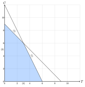
Notice that our process of solving every linearly independent pair of equations resulted in all of the corner points, or basic feasible solutions, of the Legos LP, but it also resulted in two other points: [latex](0,12)[/latex] and [latex](9,0)[/latex]. We can see in Figure 5-1 that these two points are at the intersections of two constraint boundaries, but they are not in the feasible region. We can see observe both geometrically and algebraically that [latex](9,0)[/latex] violates constraint (1) and [latex](0,12)[/latex] violates constraint (2).
The points that are found at the intersections of constraints, such as the six that we found in the table above for the Legos problem, are called basic solutions.
The process described above leads us to the following algorithm for solving linear programs with bounded feasible regions.
Corner Point Algorithm (to Solve an LP)
Suppose linear program (P) has a bounded, nonempty feasible region. Further suppose that (P) has decision variables. To solve (P):
- Find all sets of d linearly independent constraints of (P)
- Solve each of the corresponding x linear systems, arriving at a set of basic solutions, S
- Test each basic solution in S for feasibility, eliminating the infeasible basic solutions. The remaining set of solutions, B, the set of basic feasible solutions, or corner points, of the feasible region.
- Evaluate the objective function of (P) at each element of B.
- Apply Theorem 1 to identify an optimal solution to (P).
Problem 8:
Solve the LP using the Corner Point Algorithm described above:
[latex]x+y\le8[/latex]
[latex]x\ge0[/latex]
[latex]y\ge0[/latex]
[latex]z\ge0[/latex]
Solution:
The solution which maximizes the objective function is [latex](0,8,0)[/latex]. The value of the objective function at that point is 24.