10 Section II: An Application of String Art to Calculus 1
Melanie Brown; Catherine Buell; and Allison Marr
Introduction
Another engaging application of string art is in a standard Calculus I course, where we can think of each string as a tangent line to a curve. We can use a collection of tangent lines to approximate the curve; this curve forms the envelope of the tangent lines.
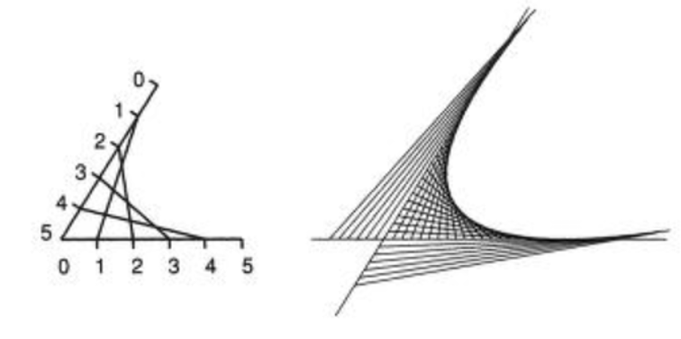
We will focus this investigation on the tangent lines of the parabola [latex]y=x^2[/latex] on a closed interval. While many authors have described activities that generate a parabola as an envelope (see Fleron et al, La Haye), this module focuses on viewing this construction as an approximation of [latex]y=x^2[/latex]. We present a research question on how close an approximation can be to the actual curve and how one can begin to conjecture and consider ways to optimize this approximation subject to different constraints. We will measure this approximation by evaluating the area between the curve and the selected tangent lines and our goal will be to try and minimize that area.
Implementation
Since this investigation does not require any additional calculus background, this investigation is appropriate to assign to a Calculus I class shortly after introducing tangent lines. Doing so provides a gentle introduction to the idea of optimization well before the traditional presentation of optimization. This investigation can also be assigned during the optimization section. However, this particular optimization problem cannot be solved with Calculus I techniques, as there are too many independent variables. Another option is to assign this investigation after learning about integration and area between curves.
Research Question
On the interval [latex]\left\lbrack-a,a\right\rbrack[/latex], where should three lines tangent to [latex]y=x^2[/latex] be placed to minimize the total area between the tangent lines and the curve?
Given that this module is appropriate for Calculus I students who have just completed tangent lines and differentiation rules, the measurement of the area is determined for students using Desmos software. The description of the application is below; however, this question could also be posed to students after studying areas between curves without immediately introducing the software. It is recommended, given the computational nature, that students are introduced to the Desmos software as it allows for greater levels of inquiry and exploration of the research question.
Application for Investigation
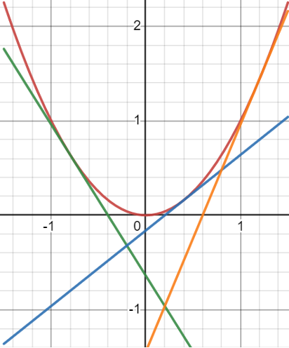
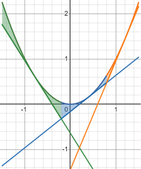
We have developed a Desmos application for this investigation available at https://www.desmos.com/calculator/o4kutwm2p4 . Students first select the value [latex]a[/latex] to set the domain interval [latex]\left\lbrack-a,a\right\rbrack[/latex]. This application has the three tangent lines defined with points of tangency at [latex]x=c[/latex], [latex]x=d[/latex], and [latex]x=f[/latex]. Students can slide values of [latex]c[/latex], [latex]d[/latex], and [latex]f[/latex] to change the value of the total area. The definitions of each of the tangent lines, as well as the corresponding areas are scripted in Desmos so that a student does not need to do any work aside from adjusting the sliders on [latex]c[/latex], [latex]d[/latex], and [latex]f[/latex]. Students do not need to compute derivatives or evaluate integrals to use this application.
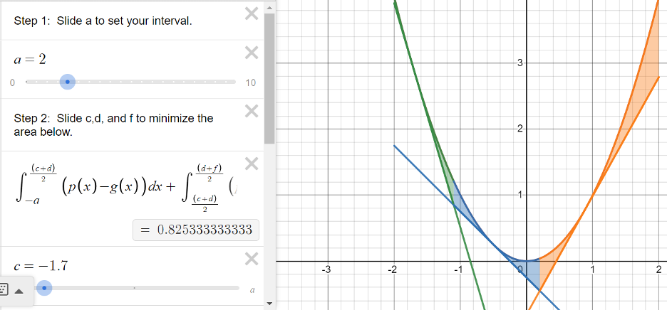
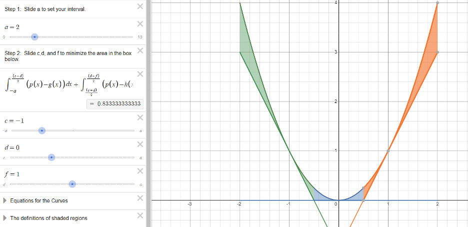
For example, if we wanted to explore this question on the closed interval [latex]\left\lbrack-2,2\right\rbrack[/latex], we would first adjust the slider on a to set it to [latex]a=2[/latex]. We might naively begin with tangent lines at [latex]c=-1[/latex], [latex]d=0[/latex], and [latex]f=1[/latex]. The calculator gives a resulting area of 0.833.
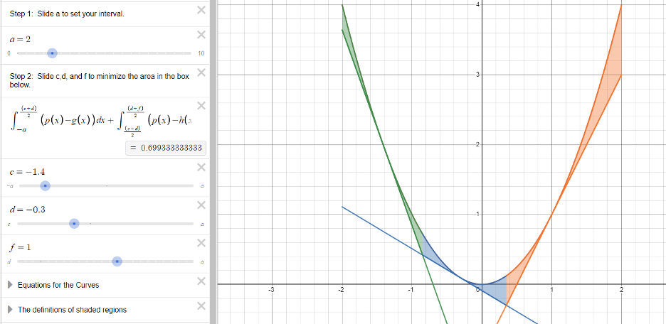
However, if we change the [latex]c[/latex] to -1.4 and [latex]d[/latex] to -0.3 and keep [latex]f=1[/latex], the total area is now 0.699.
We can continue to manipulate these values until we have convinced ourselves through either trial-and-error or mathematical logic that we have the smallest total area.
Suggested Scaffolding for Research Question
- Have students continue the investigation based on the example of [latex]\left\lbrack-2,2\right\rbrack[/latex]. Is there a consensus on the best picks for [latex]c[/latex], [latex]d[/latex], and [latex]f[/latex]? What is the minimum value?
- Let’s all change the slider of [latex]a[/latex] to 1 and consider [latex]\left\lbrack-1,1\right\rbrack[/latex]. What about now?
- Do you have any conjectures for [latex]\left\lbrack-3,3\right\rbrack[/latex]? Let’s test it.
- Let students choose a bound and gather more information. Consider open-ended questions like:
- Do we have a conjecture for the placement of values for the interval [latex]\left\lbrack-a,a\right\rbrack[/latex] and the minimized area between? What tools might we need to check this conjecture?
- What are some limitations to this software? What do you wish you could do?
(answers might include changing the function to a translation of the [latex]y=x^2[/latex] or having four or five tangent lines.)
Potential Modifications to the Desmos Code:
Parameters: The slider on [latex]a[/latex] has a step value of 0.5 and the sliders for [latex]c[/latex], [latex]d[/latex], and [latex]f[/latex] have a step value of 0.1. Additionally, the slider on [latex]c[/latex] is set to have [latex]a[/latex] as a lower bound, and the slider on [latex]d[/latex] is set such that [latex]c[/latex] is the lower bound and [latex]f[/latex] is the upper bound. Similarly, the slider on [latex]f[/latex] is set to have [latex]d[/latex] as a lower bound and [latex]a[/latex] as an upper bound. Instructors are welcome to modify these specifications as desired.
Functions: This exploration avails itself of the symmetry of [latex]y=x^2[/latex]. Any changes to the function being approximated will require redefining the tangent lines and recalculating the intersection points for the tangent lines. For [latex]y=x^2[/latex], the lines tangent to the curve at [latex]x=c[/latex] and [latex]x=d[/latex] will always intersect at [latex]x=\frac{c+d}{2}[/latex]. The tangent line at [latex]x=c[/latex] has the form [latex]y=2cx-c^2[/latex].
Extensions
While student questions might generate future directions, below are some possible considerations for students beyond a Calculus I course.
- Different number of tangent lines: The principles behind the Desmos app development will be the same, so it will not take much to scale up to four, five, or even more lines so long as you continue with [latex]y=x^2[/latex].
- Arc length: A different way of measuring how close the tangent line approximation is to the given function is comparing the arc length of the function with the sum of the line segment lengths. Such an extension would be appropriate for a Calculus II class or an independent research student.
- Different function: We selected [latex]y=x^2[/latex] for several reasons. Parabolas are well-studied curves and have myriad additional properties, and this investigation was greatly simplified because a parabola is symmetric across its axis. A similar investigation around an extremum of a different function could prove interesting.
Glossary
Envelope
A curve that touches each member of a family of curves tangentially. In other words, for a given family of curves, the envelope touches each member one tangentially.
Optimization
The action of making the best or most effective use of a situation or resource.
References
Fleron, J.; Hotchkiss, P.; von Renesse, C. Discovering the Art of Mathematics: Ideas of Calculus. (September 2015 version) http://www.artofmathematics.org/books/.
La Haye, R. String Art in a First Calculus Course. Primus 2016, 26 (4), 274–282 DOI: 10.1080/10511970.2015.1124302.
Wells, D. G. The Penguin Dictionary of Curious and Interesting Geometry; Penguin Book; Penguin Books: London, England, 1991.