7 The Algebra of a Linear Program
James Kupetz; Earl Lee; Karl Levy; and Daphne Skipper
Imagine this simple example:
A company manufactures two products, A and B. Product A sells for $10 of profit and product B sells for $12. The company has three departments which the products pass through. Department 1 requires 4 hours for each product A and product B. There are 600 hours of labor available in this department. Department 2 requires 3 hours for each product A and 2 hours for a product B. This department has 500 hours available. Department 3 requires 2 hours for each product A and 4 hours for product B. There are 500 hours available in this department
| Department | Hours / Product A | Hours / Product B | Available hours |
|---|---|---|---|
| 1 | 4 | 4 | 600 |
| 2 | 3 | 2 | 500 |
| 3 | 2 | 4 | 500 |
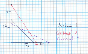
If [latex]x_a[/latex] and [latex]x_b[/latex] are the number of products A and B to be manufactured, the total profit (which we will call [latex]z[/latex] is [latex]10x_a[/latex] and [latex]12x_b[/latex]. But the process has a set of requirements, referred to as constraints. The hours of labor available in each department cannot be violated.
For Department 1:
[latex]4x_a+4x_b\le600[/latex]
For Department 2:
[latex]3x_a+2x_b\le500[/latex]
For Department 3:
[latex]2x_a+4x_b\le500[/latex]
The algebra for this is:
[latex]3x_a+2x_b\le500[/latex]
[latex]2x_a+4x_b\le500[/latex]
[latex]x_a,x_b\ge0[/latex]
Let’s start with some definitions.
A linear program is in standard form if:
- It is a minimization problem;
- With equality constraints;
- And all variables are non-negative.
[latex]z\ge0[/latex]
How is the production problem converted to standard form?
Converting from maximization to minimization:
Maximizing [latex]c^Tx[/latex] is equivalent to minimizing [latex]-c^Tx[/latex] subject to [latex]x[/latex] being feasible in both cases. Keep in mind, [latex]y-c^Tx[/latex] is a reflection of [latex]y=c^Tx[/latex], so a maximum in one becomes a minimum in the other.
Converting the inequalities to equality constraints:
For each inequality constraint, a slack variable will be introduced. This slack variable must also be non-negative values. The slack variables will be [latex]u[/latex], [latex]v[/latex], and [latex]w[/latex].
The inequality [latex]4x_a+4x_b\le600[/latex] becomes:
[latex]4x_a+4x_b+u=600[/latex]
The inequality [latex]3x_a+2x_b\le500[/latex] becomes:
[latex]3x_a+2x_b+v=500[/latex]
The inequality [latex]2x_a+4x_b\le500[/latex] becomes:
[latex]2x_a+4x_b+w=500[/latex]
where [latex]x_a,x_b,u,v,w\ge0[/latex]
A good practice when solving linear programs is to have all variables on the left side of the equation and constants on the right side.
Converting to standard form, the production problem has become:
[latex]3x_a+2x_b=500[/latex]
[latex]2x_a+4x_b=500[/latex]
And using linear algebra and matrix notations, this would look like
[latex]z\ge0[/latex]

How is the production problem converted to standard form?
These matrices are:
A: the set of coefficients of the constraints
| [latex]x_a[/latex] | [latex]x_b[/latex] | [latex]u[/latex] | [latex]v[/latex] | [latex]w[/latex] |
| 4 | 4 | 1 | 0 | 0 |
| 3 | 2 | 0 | 1 | 0 |
| 2 | 4 | 0 | 0 | 1 |
b: the constants for each constraint
| 600 |
| 500 |
| 500 |
cT: the coefficients of the objective
| -10 | -12 | 0 | 0 | 0 |
d: the constant from the objective function
At this point we form the simplex tableau
| cT | –d |
| A | b |
| eqn 4 | -10 | -12 | 0 | 0 | 0 | 0 |
| eqn 1 | 4 | 4 | 1 | 0 | 0 | 600 |
| eqn 2 | 3 | 2 | 0 | 1 | 0 | 500 |
| eqn 3 | 2 | 4 | 0 | 0 | 1 | 500 |
New Definition
Each constraint contains one variable with a coefficient of 1 that does not appear in any other constraint or the objective. Each variable that meets this condition is called a basic variable. The others are called non-basic variables. For this problem, [latex]x_a[/latex] and [latex]x_b[/latex] are non-basic and [latex]u[/latex], [latex]v[/latex], and [latex]w[/latex] are basic variables. If basic row operations can not be used to get the problem into canonical form, then the problem is infeasible.
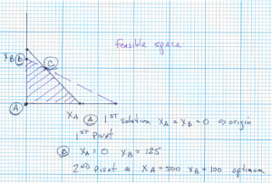
If the non-basic variables are set to 0, then the following feasible solution can be determined by inspection.
[latex]u=600[/latex]
[latex]v=500[/latex]
[latex]w=500[/latex]
[latex]x_a=x_b=0[/latex]
And the objective value is 0. This makes sense since no products are being produced, so there would be no profit.
The goal is to find the smallest value of the objective [latex]\left(z\right)[/latex] that satisfies the constraints. Since the coefficients of both [latex]x_a[/latex] and [latex]x_b[/latex] are negative, any increase in their value will reduce the objective. But how much can either be increased? Begin by choosing [latex]x_b[/latex] since it has the more negative coefficient.
Each constraint must remain non-negative.
[latex]4x_b+u\le600[/latex] or [latex]u\le600-4x_b[/latex]
[latex]3x_b+v\le500[/latex] or [latex]v\le500-3x_b[/latex]
[latex]4x_b+w\le500[/latex] or [latex]w\le500-4x_b[/latex]
Keep [latex]u[/latex], [latex]v[/latex], and [latex]w[/latex] non-negative, and limit [latex]x_b[/latex] at 125 (based on the third equation).
Row operations will be performed to make the coefficient of [latex]x_b=1[/latex] in constraint 3 and then remove [latex]x_b[/latex] from the other constraints and the objective.
Equation 3: [latex]2x_a+4x_b+w=500[/latex]
Divide by 4: [latex].5x_a+x_b+.25w=125[/latex]
Call the resulting equation 3A
Remove [latex]x_b[/latex] from Equation 1
Equation 1: [latex]4x_a+4x_b+u=600[/latex]
–4 times equation 3A: [latex]-2x_a-4x_b-w=-500[/latex]
Results in Equation 1A: [latex]2x_a+u-w=100[/latex]
Remove [latex]x_b[/latex] from equation 2
Equation 2: [latex]3x_a+2x_b+v=500[/latex]
–2 times equation 3A: [latex]-x_a-2x_b-.5w=-250[/latex]
Results in Equation 2A: [latex]2x_a+v-.5w=250[/latex]
Remove [latex]x_b[/latex] from the objective (equation 4)
Equation 4: [latex]-10x_a-12x_b=0[/latex]
12 times Equation 3A: [latex]6x_a+12x_b+3w=1500[/latex]
Results in Equation 4A: [latex]-4x_a+3w=1500[/latex]
Which gives the following new simplex tableau:
| eqn 4A | –4 | 0 | 0 | 0 | 3 | 1500 |
| eqn 1A | 2 | 0 | 1 | 0 | –1 | 100 |
| eqn 2A | 2 | 0 | 0 | 1 | –0.5 | 250 |
| eqn 3A | 0.5 | 1 | 0 | 0 | –0.25 | 125 |
[latex]x_b=125[/latex]
[latex]u=100[/latex]
[latex]v=250[/latex]
[latex]x_a=w-0[/latex]
and the objective is at –1500
Since the coefficient of [latex]x_a[/latex] is negative, we can increase it and reduce the objective further.
[latex]2x_a+u\le100[/latex] or [latex]u\le100-2x_a[/latex]
[latex]2x_a+v\le250[/latex] or [latex]v\le250-2x_a[/latex]
[latex].5x_a+x_b\le125[/latex] or [latex]x_b\le125-.5x_a[/latex]
Keeping [latex]u[/latex], [latex]v[/latex] and [latex]x_b[/latex] non-negative, [latex]x_a[/latex] is limited to 50. (first equation)
Repeat the process to make the coefficient of [latex]x_a=1[/latex] and remove it from the other constraints and objective:
Equation 1A: [latex]2x_a+u-w=100[/latex]
Divide by 2: [latex]1x_a+.5u-.5w=50[/latex]
Call the resulting equation 1B
Next:
Equation 2A: [latex]2x_a+v-.5w=250[/latex]
–2 times equation 1B: [latex]-2a_x-u-w=-100[/latex]
Results in Equation 2B: [latex]-u+v-1.5w=150[/latex]
Then:
Equation 3A: [latex].5x_a+x_b+25w=125[/latex]
–.5 times equation 1A: [latex]-.5x_a-.25u-.25w=-250[/latex]
Results in Equation 3B: [latex]x_b-.25w=100[/latex]
Remove [latex]x_a[/latex] from the objective (equation 4)
Equation 4A: [latex]-4x_a+3w=1500[/latex]
4 times Equation 1A: [latex]4x_a+2u-2w=200[/latex]
Results in Equation 4B: [latex]2u+w=1700[/latex]
Which gives a revised simplex tableau:
| eqn 4B | 0 | 0 | 2 | 0 | 1 | 1700 |
| eqn 1B | 1 | 0 | 0.5 | 0 | -1 | 50 |
| eqn 2B | 0 | 0 | -1 | 1 | -1.5 | 150 |
| eqn 3B | 0 | 1 | 0 | 0 | -0.25 | 100 |
[latex]x_a=50[/latex]
[latex]x_b=100[/latex]
[latex]v=150[/latex]
[latex]u=w=0[/latex]
And the objective is at -1700. Since none of the coefficients of the variables in the objective are negative, this is the best that can be done. No lower value of the objective can be obtained. This is the optimal solution.

Checking the solution to the constraints:
[latex]4x_a+4x_b+u=600[/latex]
[latex]4(50)+4(100)+0=600[/latex]
[latex]3x_a+2x_b+v=500[/latex]
[latex]3(50)+2(100)+150=500[/latex]
[latex]2x_a+4x_a+w=500[/latex]
[latex]2(50)+4(100)+0=500[/latex]
