15 Quantitative Data Analysis
As discussed in Chapter 6, quantitative data consists of numbers that require statistical analysis strategies. This chapter focuses on some basic statistical techniques for analyzing the various kinds of data that quantitative methods, such as interviews, surveys, and experiments, tend to generate. Throughout this discussion, you’ll learn how researchers conduct quantitative research studies.
Overview of Quantitative Data Analysis
As with qualitative analysis, the overall goal of quantitative data analysis is to reach some conclusion by condensing large amounts of data into smaller, more manageable bits of understandable information. Quantitative methods tend to generate a relatively standardized set of data, usually stored as spreadsheets on a computer. In quantitative interviews and online surveys, the spreadsheets contain numbers indicating which respondents chose which answers to each question. In hard-copy surveys, the researcher ends up with stacks of paper surveys that need to be entered into a computer for analysis. Data from experiments tend to be in the form of pre-test and post-test surveys that respondents have answered on a computer or paper. Regardless of which forms of quantitative data the researcher ends up with, they must be prepared for statistical analysis.
As discussed in Chapter 6, most quantitative studies rely on positivist, deductive approaches based on testing existing theories. Therefore, this chapter focuses on analyzing quantitative data from a theory-testing perspective. In this type of research, quantitative data analysis entails preparing the data for analysis and using statistical techniques to test hypotheses related to the research question.
Preparing Quantitative Data for Analysis
The first step in preparing quantitative data for analysis is often getting the data into a computer program that the researcher can use for statistical analysis. If the data come in as electronic information already entered into the system by respondents, then the preparation phase is less time-consuming. This section starts with what happens when a researcher has amassed paper questionnaires. Once the questionnaires have been entered into the computer, the data preparation process looks the same for data that originally came in on paper, as it does for data that came in electronically.
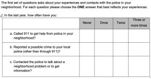
Figure 15.1 shows a snapshot of one set of questions on the hard-copy questionnaire of our policing survey. The figure shows that respondents chose one of four answer options for the three questions about their interactions with the police in the past year. You might notice no numbers are included in any of the answer choices.

Without numbers, how can a researcher statistically analyze the responses to these questions? As this example indicates, once a researcher has a stack of completed questionnaires, they must first condense the data into information represented by numbers. To do this, the researcher starts by creating a codebook, or a document that outlines how a researcher has translated their data from words into numbers.
Table 15.1 shows the section of the codebook indicating how we translated the answers from the questions in Figure 15.1 into numbers. Each row of the table relates to one question, with columns for variable names, the full text of the question, and the numbers we assigned to each answer option. The shortened variable name aids the process of data entry, providing an easy-to-read name for each question. While the answer choices on the original questionnaire had no numbers attached, the codebook indicates the numbers we chose to represent each answer choice. A researcher can assign whatever numbers they want to answer choices, but common practice is to start with 0 or 1 and move by increments of 1. In the example in Table 15.1, we started with “0” because logically, “0” means the event never happened. While consistency between the text and the number of answer choices is not required, it can help later when the researcher reads the statistical results.
Table 15.1 Example Codebook Section from Policing Survey
Variable Name |
Question |
Answer Choices |
| Call911 | In the last year, how often have you called 911 to get help from police in your neighborhood? | 0 = Never
1 = Once 2 = Twice 3 = Three or More |
| Reptcrime | In the last year, how often have you reported a possible crime to your local police (other than through 911)? | 0 = Never
1 = Once 2 = Twice 3 = Three or More |
| Contpol | In the last year, how often have you contacted the police about a neighborhood problem, or to get information? | 0 = Never
1 = Once 2 = Twice 3 = Three or More |
In preparing data for entry into the computer, the researcher’s codebook must include every piece of information on the paper questionnaire; every question and answer choice must be represented in the codebook.
Once the codebook has been created, the researcher (and any assistants) must enter the information from every paper questionnaire into a spreadsheet or data analysis program. This tedious and time-consuming process is one reason researchers might administer their survey online; if respondents have entered their answers directly into the computer, researchers can download the data and import it pre-coded into a computer program. In this case, the researcher will have created the codebook before administering the survey, so every question has a variable name, answer, and number attached to the answer when the respondents begin taking the survey online.
Manual data entry usually requires creating a spreadsheet in which each row represents one questionnaire, and each column represents a different variable (as specified by the shortened variable name explained above). Generally, the first column in the spreadsheet will be a number that identifies the questionnaire (e.g., 001, 002, etc.), so the researcher can revisit the hard-copy format if necessary. These data are entered into commonly used spreadsheet programs, such as Excel, or a specialized data analysis program such as SPSS (Statistical Package for the Social Sciences). SPSS is a statistical analysis computer program designed to analyze the type of data quantitative survey researchers collect. It can perform everything, from basic descriptive statistical analysis to more complex inferential statistical analysis. Most statistical programs, including SPSS, provide a data editor for entering data. However, these programs store data in their own native format (e.g., SPSS stores data as .sav files), which makes it difficult to share the data with other statistical programs, and researchers using different programs. Hence, researchers often enter data into a spreadsheet or database, where the information can be shared across programs, reorganized, and extracted as needed. Smaller data sets (with less than 65,000 observations and 256 items) can be stored in a spreadsheet such as Excel, while larger datasets require a database program.
Researchers who must enter their data manually have to enter the data exactly as shown in each questionnaire, or else the results of the analysis will be based on flawed data. Thus, researchers must build in time for double-checking (and sometimes triple-checking) data. In the policing survey, we had a handful of student assistants entering data. After all questionnaires had been entered into the system, we chose a random sample, roughly one-third of the questionnaires, to check for inconsistencies between the paper questionnaires and the data entered into the system. Unfortunately, we found multiple errors, leading us to recheck all 391 questionnaires. Then, just to be sure, we spot-checked another one-third of the questionnaires with the improved dataset, finding no errors. While this process took more time than anticipated, the result was a dataset that accurately represented what respondents had reported on the survey.
One issue researchers encounter when entering data is that some respondents skip questions, intentionally or inadvertently. These skipped questions become missing data, questions to which a respondent has not provided an answer. During data entry, some statistical programs automatically treat blank entries as missing values, while others require entering a specific numeric value (such as -9 or 999) to denote a missing value. Later, the researcher will determine how to handle the missing data during analysis.
Statistically Analyzing Quantitative Data
Quantitative data analysis uses statistical techniques to identify, describe, and explain patterns found in the data. Numeric data collected in a research project can be analyzed quantitatively, using statistical tools in two different ways. Descriptive analysis refers to statistically describing, aggregating, and presenting information about variables in the study. Inferential analysis refers to the statistical testing of hypotheses (theory-testing) to see if results from the sample can be generalized to a larger population. Because there are multiple statistical techniques, we cannot cover them all in one chapter. Instead, we’ll focus on descriptive statistics, which can help you get started in analyzing quantitative data, and we’ll save inferential statistics for your statistics courses.
Univariate Analysis
To start, researchers conduct univariate analysis, a statistical analysis that shows common responses and patterns across answers in one variable. (Remember how the researcher assigned each question a variable name, in the data preparation stage? That is helpful as we start to think and talk about questions as variables rather than survey questions.)
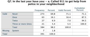
Univariate analysis includes frequency distributions and measures of central tendency. A frequency distribution is a way of summarizing the distribution of responses to a single survey question. Figure 15.2 shows a snapshot of a frequency distribution for the variable “call911” described in the example codebook entries above. I created this distribution using SPSS, and while other programs might produce frequency distributions that look different, they all contain the same elements, including a list of response options (the first column), numbers, and percentage of respondents who chose each option (the other columns).

In Figure 15.2, all response options are listed in the first column, along with row labels for the total number of respondents who answered the question (in this case, 384), the number who didn’t answer the question (7), and the overall total number of respondents (391). The “Frequency” column reports the number of respondents who answered in each response category. The “Percent” column shows the percentage of respondents who answered in each category, and the “Valid Percent” column excludes respondents who didn’t answer the question, calculating the percentage of respondents who chose each answer category. “Cumulative Percent” refers to the percent of respondents in each row, plus all the percentages in the rows above that row.
The frequency distribution of calling 911 in the past year shows the distribution of responses to the question in the survey. For example, we learn from this frequency distribution that most respondents (273 out of 391 people, or 69.8%) had not called 911 the year before the survey. We also learn that “Three or more times” was the least popular choice, with only 21 people (5.4%) saying they’d called 911 that many times in the year before the survey. You might also notice that the frequency distribution reports the answer options as categories instead of the numbers we assigned using our codebook.
In addition to helping researchers describe their data, frequency distributions can help researchers clean data. For example, the codebook for “call911” indicates that the response options should range from 0 to 3, or “Never” to “Three or More Times”. If a frequency distribution for the variable also included a row with “4” as the label, we’d know that something had gone wrong with either the data entry (the most likely), or respondents’ answers (not likely in this case, but sometimes respondents write in their answers, even when they’re asked to choose among a set of response options). In either case, the researcher would need to find that entry in the dataset and match it to the original questionnaire to figure out how to handle that response in the dataset. Running frequency distributions for every variable is an excellent way to gauge the quality of your data before conducting more complex statistical analyses.
Another form of univariate analysis that survey researchers conduct using single variables is measures of central tendency. Measures of central tendency tell us the most common or average response to a question, using three measures: modes, medians, and means. The level of measurement (see Chapter 13) determines which measures of central tendency a researcher should use for each variable. For example, the mode indicates the most common response to a question, and it’s appropriate for all levels of measurement. A frequency distribution can show us the mode. For example, in Figure 15.2, most respondents reported never having called 911 the previous year. This indicates that the modal response was 0 or “Never.”
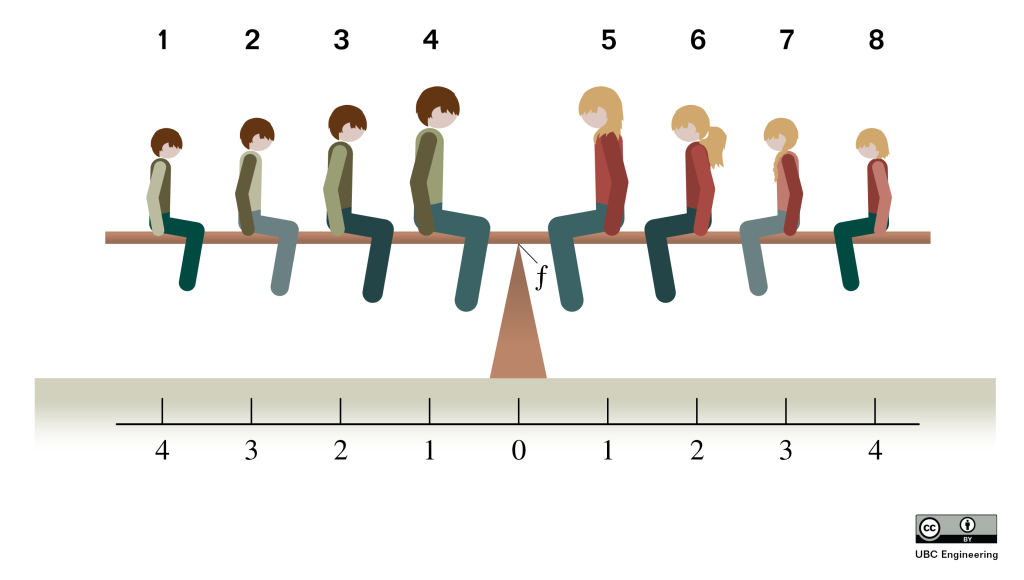
The median is the midpoint of a distribution, where half of the respondents fall on either side. Figure 15.3 illustrates one way to think about the median. In the picture, the two children balance on a central triangle, which indicates equal weight on each side of the seesaw.

The triangle in the center is similar to the median: half of the respondents would fall on the left of the triangle and half on the right to balance the seesaw. In statistical terms, 50% of responses fall on either side of the median.
The median is most appropriate for ordinal and interval/ratio-level variables. To calculate the median, we list all responses in order and choose the middle response. To find the middle point, divide the number of valid cases by two. In Figure 15.2, the number of valid cases (384) divided by 2 is 192, so we’d look in our list for the 192nd value in our distribution. That number would be our median. Luckily, we don’t have to list all 384 answers to find the median. As with the mode, we can use a frequency distribution to identify the median, as long as the distribution includes percentages ordered by numerical category. For example, Figure 15.2 presents the response options in numerical order from 0 (“Never”) to 3 (“Three or More Times”), and it includes the percentage of respondents who answered in each category. With these elements in place, we can start at the top with the “Never” row, adding up the values in the “Percent” column until the total percent tips over 50%. In this case, the first answer choice (“Never”) contains almost 70% of the answers. Seventy percent is over 50%, so we know that the midpoint of the distribution (the median) is 0 or “Never.” The cumulative percent column also shows us the median by adding the percentages automatically.
The third measure of central tendency, the mean, is what many people think of when they think of an average. The mean is the added value of all responses on a variable divided by the total number of responses. It is only appropriate for interval/ratio level variables. Because the variable we have been working on within this section is an ordinal level variable, we would be mistaken if we calculated and reported a mean. Researchers must be careful when using computer programs to calculate statistical information because these programs will calculate and return results for all measures of central tendency, regardless of the variable type. For example, when I asked SPSS to calculate a mean for the “call911” variable, it did return a result. However, knowing that the mean is not an appropriate measure of central tendency for an ordinal level variable, I would not interpret or report that result. In other words, computer programs are helpful calculators, but researchers have to decide when to use certain statistics. A researcher must be able to distinguish the appropriate statistical analyses and tests for their variables.
Bivariate and Multivariate Analysis
Researchers can learn a lot about their respondents by conducting univariate analyses of their data; they can learn even more when they examine relationships among variables. We can analyze the relationships between two variables, called bivariate analysis, or we can examine relationships among more than two variables. This latter type of analysis is known as multivariate analysis.
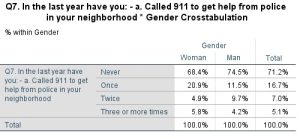
Bivariate analysis allows us to assess covariation among two variables. This means we can determine whether changes in one variable occur with changes in another. If two variables do not correlate, they are said to have independence, which means that there is no relationship between the two variables in question. To learn whether a relationship exists between two variables, a researcher may cross-tabulate the two variables and present their relationship in a contingency table. A contingency table shows how variation on one variable may be contingent upon variation on the other. Figure 15.4 shows a snapshot of a contingency table I created using SPSS. The figure shows a cross-tabulation of two questions from the policing survey: the question about calling 911 in the past year, and the respondent’s gender. (As a side note, respondents could choose “Other” as a third option under gender, but only two respondents did so, meaning we can’t use their responses for statistical analysis of differences between genders.)

In this contingency table, we can see the variable “Gender” in the table’s columns and “call911” in its rows. Typically, values contingent on other values are placed in rows (a.k.a. dependent variables), while independent variables are in columns. This makes comparing across categories of our independent variable pretty simple. For example, reading across the top row of the table, we can see that 68.4% of women reported they had never called 911 in the past year, while almost 75% of men reported the same. This result indicates that there may be some differences between how often men and women call the police. Researchers would use more advanced statistical techniques to test whether the differences seen in our contingency table can be generalized to a larger population, or if the differences are simply a result of some feature of our sample. We won’t cover those tests in this text, but you’ll learn more about them in a statistics class.
Researchers interested in simultaneously analyzing relationships among more than two variables conduct multivariate analysis. If I hypothesized that the number of times someone calls 911 declines for men as they age but increases for women, I’d consider adding age to the preceding analysis. To do so would require multivariate analysis rather than bivariate. We won’t go into detail here about conducting multivariate analysis of quantitative data, but if you’re interested in learning more about these types of analyses, consider enrolling in a statistics class. Even if you don’t aspire to become a researcher, the quantitative data analysis skills you’d develop in a statistics class could serve you well in many different careers.
Summary
- Preparing quantitative data for analysis entails creating a codebook, and then using that codebook to enter information from hard-copy questionnaires into a computer program. The data entry process also requires conducting quality checks to ensure the final dataset accurately reflects the hard-copy data.
- Codebooks for quantitative data include a variable name, the full text of the question as presented to respondents, and the numbers assigned to each answer option.
- Descriptive analysis involves statistical techniques that help the researcher describe and present information about the variables in the study. Inferential analysis involves statistical techniques that help the researcher test hypotheses to see if sample results can be generalized to a broader population.
- Univariate analysis focuses on one variable; bivariate analysis focuses on two variables; multivariate analysis focuses on more than two variables.
- Frequency distributions show the distribution of responses to a single variable. They include a list of response options and the number or percent of respondents who chose each option.
- The mean, median, and mode are all measures of central tendency. The mean is the numerical average of all responses, used for
interval/ratio level variables. The median is the midpoint of a distribution of responses, used for ordinal and interval/ratio variables. The mode is the most common response for nominal, ordinal, and interval/ratio variables. - Contingency tables show how variation on one variable may depend on variation of another. They include response options for one variable (usually the independent variable) in the columns, and options for the other variable in rows. The middle of a contingency table shows the percentage of respondents who answered within each combination of response options.
Key Terms
| Bivariate Analysis | Frequency Distribution | Median |
| Codebook | Independence | Missing Data |
| Contingency Table | Inferential Analysis | Mode |
| Covariation | Mean | Multivariate Analysis |
| Descriptive Analysis | Measures of Central Tendency | Univariate Analysis |
Discussion Questions
- What challenges might a researcher run into when preparing quantitative data for analysis? How would the challenges be different for online questionnaires versus hard-copy questionnaires?
- Create three closed-ended questions that you might use in an interview, survey, or pre-test and post-test during an experiment. Then, develop a codebook for those three questions. How did you decide what to name your variables? How did you decide what numbers to attach to your answer choices?
- Pretend you’ve asked 100 people to answer the three questions you developed for question 2. Create a frequency distribution based on their hypothetical responses. Then, interpret the numbers in your frequency distribution.
- Identify the measure(s) of central tendency appropriate for analyzing each variable described in your frequency distribution from question 3. How do you know whether to use mean, median, or mode for each variable? As a bonus, see if you can calculate the appropriate measure(s) of central tendency for each variable.
- How do you think the answers to your three questions are different between people under 65 years old and people 65 and older? Create and interpret a contingency table to explain your answer to this question.
Media Attributions
- Figure 15.1 Policing Survey Question 1 as Presented on the Questionnaire © Williams, Monica is licensed under a CC BY-NC-SA (Attribution NonCommercial ShareAlike) license
- Figure 15.2 Univariate Frequency Distribution © Williams, Monica is licensed under a CC BY-NC-SA (Attribution NonCommercial ShareAlike) license
- Figure 15.3 Illustration of a Median © Brina Schenk with UBC and Douglas College is licensed under a CC BY (Attribution) license
- Figure 15.4 Bivariate Contingency Table © Williams, Monica is licensed under a CC BY-NC-SA (Attribution NonCommercial ShareAlike) license

