College of Science
107 Mathematical Models of SARS-CoV-2 Testing: Explaining Differences in Test Results Among Patients
Muskan Walia and Frederick R. Adler
Faculty Mentor: Frederick R. Adler (School of Biological Sciences and Mathematics, University of Utah)
1. Introduction
At the onset of the pandemic, testing was used primarily for surveillance purposes to assess the prevalence of COVID-19 in communities. We understood that, in relation to public health- oriented goals, no test is perfect; every test makes mistakes. Some tests return a negative result if someone is infected. These are called false negatives, and a test which produces them is said to have imperfect sensitivity. On the other hand, some people who are not infected test positive. These results are called false positives, and such a test is said to have imperfect specificity [14]. Moreover, heterogeneity within populations makes tests difficult to interpret.
Being five years into the pandemic, rather than administering tests at a testing center for surveillance purposes, tests are predominantly used in hospitals, clinics, and at home as decision tools. In hospitals, tests inform choice of care and isolation protocols, while tests at home influence only our personal response about masking and isolation protocols. Current CDC guidelines recommend people quarantine for at least five days after a positive test. Protocols, like isolation, as a result of a positive COVID test have been modeled at the population level considerably throughout the course of the pandemic [5, 2]. However, we are interested in studying the testing mechanisms at the level of an individual. These CDC isolation recommendations utilize both symptoms and physical COVID-19 tests to predict infectiousness. Using these tests, whether symptoms or physical tests, to help ascertain and track infectiousness can then help facilitate effective measures to limit the transmission of infection. Unfortunately, many have reported lingering positive test results when they are no longer symptomatic or infectious, causing hesitation and unnecessary isolation and disruption to personal lives. Specifically, multiple studies have demonstrated that PCR tests may continue to yield positive results even after an individual is no longer infectious, due to lingering RNA fragments [9, 3, 8]. Antigen tests, while generally less sensitive, may better reflect a person’s infectivity because they correlate more closely with viral culture positivity [13, 11].
However, for both test types, it is known that the timing of a test relative to the course of infection affects the results [4]. In other words, the probability of a true positive depends on the stage of the infection. However, this infection timeline varies amongst individuals in a population and there are questions about the sources of this variation. The components of variation are initial virus dose, body size, rate of the spread of infection in the body, and clearance. To help address this question about variation, we developed a dynamical model using the aforementioned components of variation to describe the course of infection and when an individual tests positive in that infection timeline. We also utilize this model to conduct a sensitivity analysis, that is, an assessment of which model parameters influence the course of infection the most. We then compare this testing model results to a statistical model of symptoms, where we use symptoms as a test.
2. Methods
2.1 Virus dynamics and testing model
Throughout the course of the pandemic, epidemiologists have relied heavily upon the Susceptible-Infected-Recovered (SIR) Model, which uses differential equations to model contagion spread in a population. Because we are studying COVID-19 tests, we must model what happens inside of people rather than the spread of infection throughout a population. Conveniently, SIR models can be used to study what happens at the cellular level in the upper respiratory tract when people become infected. Our extension of the SIR model describes the dynamics of how cells transition between the states, produce viruses, and generate the dead viruses and cells (detritus) that tests detect even after the infection has been cleared (figure 1). We initialize the model with 0 infected cells and 100 viruses because when we contract an infection, we inhale viral particles, not cells. Once the infection is contracted, the viral replication process is initiated.
The Deterministic SIVRD Model
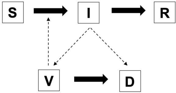
Figure 1. The structure of the SIVRD Model. Susceptible Cells (S) become infected cells (I) and can recover (R). Infected cells can generate viruses (V), which can infect susceptible cells. Tests detect detritus (D) produced by infected cells or viruses.
The biological model of the infection we created can be described by the system of equations.
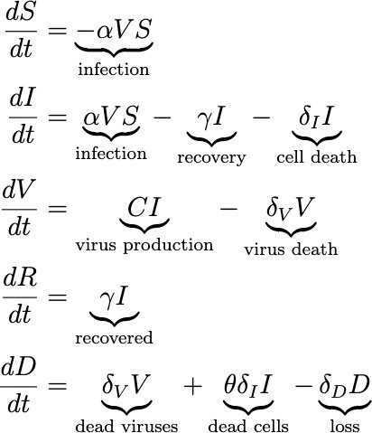
These equations describe the dynamics of how susceptible cells get infected by viruses, produce viruses, and then die or recover. As cells and viruses die, they produce the detritus that is detectable by tests. We then include W(t) to model the process of sampling for an antigen test, where W(t) represents the total expected number of detectable viruses we would collect in a testing sample, defined by:

where nI, nV , and nD represent the number of detectable RNA sequences obtained from infected cells, virus, and detritus and I, V , and D represent the fraction of viruses and detritus that survives the collection and processing.
After meeting with testing experts at two local companies, ARUP and BioFire, to understand the make-up of a testing sample and testing process, we received estimates for the values of and n and extrapolated that the volume fraction that is collected for a testing sample is = 0.01. W(t) could be detected as SARS-CoV-2 by the test and, therefore, output a positive result.
The Stochastic SIVRD Model
Randomness is inherent in the course of an infection. So, we can create a stochastic version of the SIVRD model to include this variation. We ran stochastic simulations for these equations using Binomial and Poisson approximations in an Euler’s scheme. The Binomial describes the probabilities of different transitions of cells, and the Poisson describes the count of different events. Euler’s scheme introduces a time step, T. The system of equations is given by:
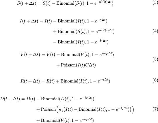

The deterministic model represents the expectation of the stochastic process. However, the individual runs of the stochastic process deviate from the mean because of randomness. The goal is to have the stochastic and deterministic models align to ensure that the deterministic model provides a useful approximation of a truly stochastic process.
For both the deterministic and stochastic models, we simulated the entire course of infection (from day 0 to day 30) with a small timestep of .01 for each. We do not include cell regrowth. We ran the simulation 1000 times, stored them in distinct data frames, and then averaged those 1000 simulations.
2.2 Symptom Model
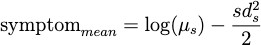
After finalizing these biological and testing models, we built a symptom model, a statistical model that inputs symptom duration and symptom onset data from a cohort of patients, calculated the mean, median, and standard deviation, and then used those values to create a lognormal distribution modeling the probability of symptoms, and therefore ‘testing’ positive, at various times of the infection [10]. We fit a lognormal distribution with a matching mean and variance. To determine the parameters of the lognormal distribution from the observed mean and variance, we use the following equations:

We then overlaid this symptom model with the results from the deterministic and stochastic models above.
Variability can arise from measurable factors or stochastic processes. However, our simulation lacks true stochasticity, meaning our results are entirely determined by parameter values. To explain the observed variance, we use the aforementioned data frames to perform a transformed linear regression, identifying which parameters on each day account for the most variation between patients. By analyzing trends across days, we demonstrate that the parameters with explanatory value change over time.
Parameter Estimation
Table 1. Model parameters along with justifications and references.
|
Parameter |
Description (unit) |
Value |
Justification and References |
|
R0 |
Basic reproduction number (unitless) |
7.4 |
Ke et al.[7] |
|
12.32 |
Marc et al.[12] |
||
|
R0,cv |
Coefficientof variation of R0 (unitless) |
0.25 |
Estimated |
|
S0,mean |
Initial susceptible cells (cells) |
1010 |
There are approximately 3 · 1013 totals cells in the body. 1/30 of those total cells are viable to get infected. Realistically, S0,mean = 1012. For numerical reasons, we use S0,mean = 1010. |
|
S0,cv |
Coefficient of variation of S0,mean (unitless) |
0.25 |
Estimated |
|
|
Clearance rate of infected cells |
0.5/day |
Infected cells assumed to last ~2 days. [15] |
|
|
Coefficientof variationof 𝛿𝐼,𝑚𝑒𝑎𝑛 (unitless) |
0.25 |
Estimated |
|
|
Clearance rate of viruses |
22.31/day |
Some studies suggest that inhaling 100–800 virions may initiate infection. Other research indicates that the infectious dose could be as low as 100 viral particles [6]. |


|
|
Coefficientof variationof 𝛿𝑉,𝑚𝑒𝑎𝑛 (unitless) |
0.25 |
Estimated |

|
V0,mean |
Initialviral load (virions) |
100 |
Some studies suggest that inhaling between 200 and 800 infectious virions may be sufficient to initiate an infection. Other research indicates that the infectious dose could be as low as 100 viral particles [6]. |
|
V0,cv |
Coefficient of variation of V0,mean (unitless) |
0.25 |
Estimated |
|
C |
Burst size |
102 |
Middle of estimated range (10– 10,000) from Grebennikov et al.[1] |
|
|
Clearance rate of detritus |
0.5/day |
Estimate of 0.14/day produced unrealistic results [17]. |
|
|
Coefficientof variationof 𝛿𝐷,𝑚𝑒𝑎𝑛 (unitless) |
0.25 |
Estimated |

|
|
Virusequivalents produced by dying cell (unitless) |
0.1 |
Estimated |
|
|
Fraction of infected fluidcollected (unitless) |
0.0001 |
Estimate from an interview with ARUP and BioFire staff. |
|
|
Fractionof collected infected cells that survive after the test sample is processed (unitless) |
10 4 |
Estimate from an interview with ARUP and BioFire staff. |
|
|
Fractionof collected viruses that survive after the test sample is processed (unitless) |
10 4 |
Estimate from an interview with ARUP and BioFire staff. |


|
|
Fractionof collected detritus that survives after the test sample is processed (unitless) |
10 4 |
Estimate from an interview with ARUP and BioFire staff. |

|
nI |
Numberof detectable RNA sequences per cell |
30 |
Estimate from an interview with ARUP and BioFire staff. |
|
nV |
Numberof detectable RNA sequences per virus |
1 |
Estimate from an interview with ARUP and BioFire staff. |
|
nD |
Numberof detectable RNA sequences per unit detritus |
0.5 |
Estimate from an interview with ARUP and BioFire staff. |
|
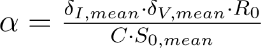
|
Infection rate per virus per cell |
Estimated from R0 |
|

|
|
Coecientof variation of ↵mean |
0.25 |
Estimated |
|
totalT |
Length of infection (days) |
30 |
Estimated |
|
|
Simulation timestep (days) |
0.1 |
Estimated |


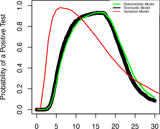
Results
Figure 2 illustrates the dynamics of the variables for 20 individuals in the deterministic and stochastic models. We do not include a graph of R because it does not feed back to the results. In the graph for W, the total expected number of detectable viruses in a testing sample, we include a horizontal line at log10(60). This threshold represents the detection limit of the test
— when the viral content in a sample exceeds this value, the test is assumed to return a positive result.
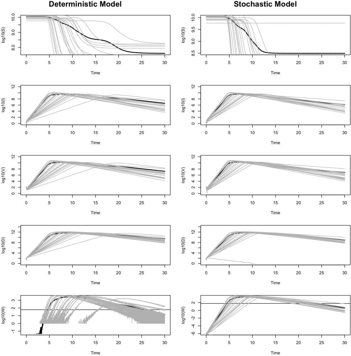
Figure 2. Dynamics of the deterministic and stochastic SIVRD model for 20 patients. Each thin gray line represents an individual patient, and the thick black line is the average of all patients. All results are presented as log base 10.
The final model, seen in figure 3, reveals that people can test negative even when they are still infected. This could be explained for different reasons depending on if they are earlier or later in their course of infection. Moreover, there exists substantial variation in the timing of positive tests due to differences between people. The overlaid model also illustrates that symptoms persist longer than positive antigen tests. We are able to show that neither antigen tests nor symptom models provide a perfect prediction of infectiousness, particularly when people’s course of infection varies.
Days Since Infection
Figure 3. Results from the SIVRD model. We compare the probability of a positive test in a population of patients with the deterministic model (green curve), stochastic model (black dots), and the symptom model (red curve).
In the literature, we find that I, representing the rate of infected cell clearance, is an uncertain parameter, with values ranging from 0.1 to 1.2 [7, 16]. Similarly, R0 has estimated values of 7.4 and 12.32 in different studies [7, 12]. Furthermore, the results of our models are sensitive to the values of I and R0. To assess the impact of this uncertainty and sensitivity, we simulate model outputs across three representative values of I (0.1, 0.5, and 1.2) and R0 (set at 7.4 and 12.32) and assess the effects on the predicted probability of a positive test over time.
Figure 4 displays the output of our deterministic model (green), stochastic model (black), and a symptom-based model (red) across these parameter regimes. The symptom model remains unchanged across parameter variations because it does not depend on I or R0. For the deterministic and stochastic models, we find that both I and R0 strongly influence the shape and timing of the predicted test positivity curves.
At low I values, the probability of testing positive increases slowly over time. In contrast, higher values of I result in sharper peaks and shorter durations of test positivity. This suggests that faster clearance rates (higher I) lead to a smaller window of detectability.
Moreover, increasing R0 leads to an earlier and more pronounced peak in positivity, reflecting a faster-growing infection.
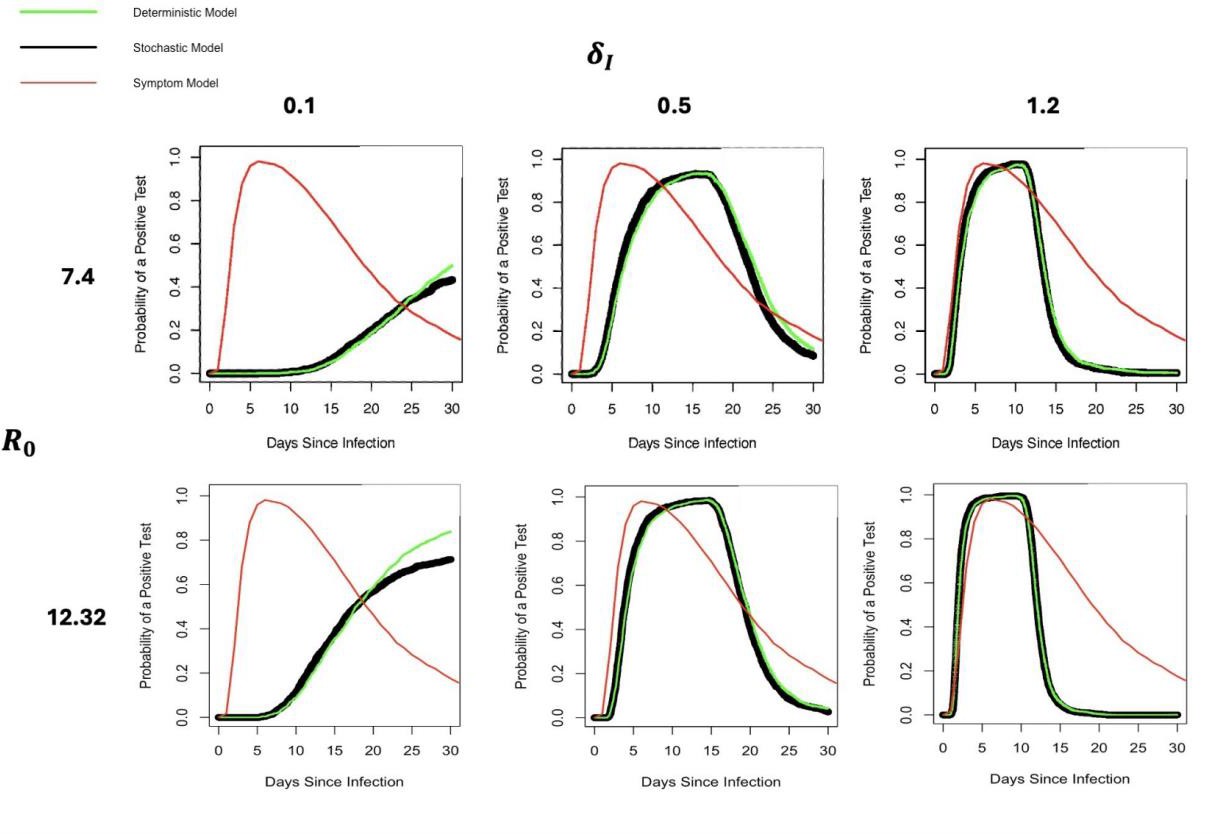
Figure 4. Effects of R0 and I parameter values on the probability of a positive test. Notation as in figure 3.
Discussion
Throughout the COVID-19 pandemic, many have observed puzzling variability in test results: some individuals seem to test positive for extended periods, others never test positive despite symptoms or exposure, and some test negative throughout their infection. We hypothesize that these differences may be attributable to individual biological variability. Specifically, we predict that differences in viral kinetics influence early test outcomes, while differences in immune response impact the duration of positivity in the later stages of infection. To test this, we created a dynamical model using components of variation in individuals such as initial virus dose, body size, rate of spread of infection in the body, and clearance to describe the course of infection. We utilize this model to conduct a sensitivity analysis, that is, an assessment of which model parameters influence the course of infection the most. We then compare this testing model results to a statistical model of symptoms, where we use symptoms as a test.
We are able to show that neither antigen tests nor symptom models provide a perfect prediction of infectiousness, particularly when people’s course of infection varies. Our models help explain the causes of imperfect specificity of SARS-CoV-2 tests. This is useful for practitioners and, as a future application, can be verified by them because our research process involved practitioners, like ARUP, and our modeling framework is generalizable because our models were built on actual mechanisms and idealized population parameters.
A limitation of our model is its specificity to a particular diagnostic test—the one administered by ARUP. Evidently, many different COVID-19 tests exist, each with varying thresholds for what constitutes a positive result. These thresholds depend on the test type, the components present in the sample, and the sample’s dynamics. As an extension of our work, the model could be adapted to reflect the characteristics and sensitivity of other tests to broaden its applicability.
Another limitation of our approach is that we do not explicitly model the immune response, and therefore assume parameters such as clearance rates remain constant over the course of an infection within an individual. If biomarkers indicative of a strong immune response (i.e., a high I) could be identified and measured, they would offer a compelling foundation for extending our model. Incorporating such data could improve predictions of prolonged test positivity and help public health officials tailor isolation guidelines and testing strategies—particularly for individuals whose immune systems clear infection more slowly.
References
[1] Dmitry Grebennikov, Elena Kholodareva, Igor Sazonov, Anastasia Karsonova, Andreas Meyerhans, and Gennady Bocharov. Intracellular life cycle kinetics of sars-cov-2 predicted using mathematical modelling. Viruses, 13(9):1735, Aug 31 2021.
[2] KE Hanson, AM Caliendo, CA Arias, MK Hayden, JA Englund, MJ Lee, et al. The infectious diseases society of america guidelines on the diagnosis of covid-19. Molecular diagnostic testing 2020 [cited 2020 september 12].
[3] Chung-Guei Huang, Kuo-Ming Lee, Mei-Jen Hsiao, Shu-Li Yang, Peng-Nien Huang, Yu-Nong Gong, Tzu-Hsuan Hsieh, Po-Wei Huang, Ya-Jhu Lin, Yi-Chun Liu, et al. Culture-based virus isolation to evaluate potential infectivity of clinical specimens tested for COVID-19. Journal of Clinical Microbiology, 58, 2020.
[4] Romney M Humphries, Marwan M Azar, Angela M Caliendo, Andrew Chou, Robert C Colgrove, Valeria Fabre, Christine C Ginocchio, Kimberly E Hanson, Mary K Hayden, Dylan R Pillai, et al. To test, perchance to diagnose: Practical strategies for severe acute respiratory syndrome coronavirus 2 testing. 8:ofab095, 2021.
[5] Katherine F Jarvis and Joshua B Kelley. Temporal dynamics of viral load and false negative rate influence the levels of testing necessary to combat covid-19 spread. Scientific reports, 11(1):1–12, 2021.
[6] Shirin Karimzadeh, Raj Bhopal, and H. Nguyen Tien. Review of infective dose, routes of transmission and outcome of covid-19 caused by the sars-cov-2: comparison with other respiratory viruses. Epidemiology and Infection, 149:e96, 2021.
[7] Ruian Ke, Carolin Zitzmann, David D Ho, Ruy M Ribeiro, and Alan S Perelson. In vivo kinetics of SARS-CoV-2 infection and its relationship with a person’s infectiousness. Proceedings of the National Academy of Sciences, 118:e2111477118, 2021.
[8] Min-Chul Kim, Chunguang Cui, Kyeong-Ryeol Shin, Joon-Yong Bae, Oh-Joo Kweon, Mi-Kyung Lee, Seong-Ho Choi, Sun-Young Jung, Man-Seong Park, and Jin-Won Chung. Duration of culturable SARS-CoV-2 in hospitalized patients with COVID-19. New England Journal of Medicine, 384:671–673, 2021.
[9] Lauren M Kucirka, Stephen A Lauer, Oliver Laeyendecker, Denali Boon, and Justin Lessler. Variation in false-negative rate of reverse transcriptase polymerase chain reaction–based sars-cov-2 tests by time since exposure. Annals of internal medicine, 173(4):262–267, 2020.
[10] Alexandra Lane, Krystal Hunter, Elizabeth Leilani Lee, Daniel Hyman, Peter Bross, Andrew Alabd, Melanie Betchen, Vittorio Terrigno, Shikha Talwar, Daniel Ricketti, Bennett Shenker, Thomas Clyde, and Brian W Roberts. Clinical characteristics and symptom duration among outpatients with covid-19. American Journal of Infection Control, 50(4):383–389, 2022.
[11] Brian Le↵erts. Antigen Test Positivity After COVID-19 Isolation—Yukon-Kuskokwim Delta Region, Alaska, January–February 2022. MMWR. Morbidity and Mortality Weekly Report, 71, 2022.
[12] Aur´elien Marc, Marion Kerioui, Fran¸cois Blanquart, Julie Bertrand, Oriol Mitja`, Marc Corbacho-Monn´e, Michael Marks, and J´er´emie Guedj. Quantifying the relationship between SARS-CoV-2 viral load and infectiousness. medRxiv, 2021.
[13] Andrew Pekosz, Charles Cooper, Valentin Parvu, Maggie Li, Je↵rey Andrews, Yukari CC Manabe, Salma Kodsi, Je↵ry Leitch, Devin Gary, and Celine Roger-Dalbert. Antigen-based testing but not real-time PCR correlates with SARS-CoV-2 virus culture. medRxiv, 2020.
[14] Alan S Perelson and Ruian Ke. Mechanistic modeling of sars-cov-2 and other infectious diseases and the e↵ects of therapeutics. Clinical Pharmacology & Therapeutics, 109(4):829–840, 2021.
[15] Alan S. Perelson, Avidan U. Neumann, Martin Markowitz, James M. Leonard, and David D. Ho. Hiv-1 dynamics in vivo: virion clearance rate, infected cell life-span, and viral generation time. Science, 271(5255):1582–1586, 1996.
[16] Steven Sanche, Tyler Cassidy, Pinghan Chu, Alan S Perelson, Ruy M Ribeiro, and Ruian Ke. A simple model of COVID-19 explains disease severity and the e↵ect of treatments. Scientific Reports, 12:1–14, 2022.
[17] Mark J Siedner, Julie Boucau, Rebecca F Gilbert, Rockib Uddin, Jonathan Luu, Sebastien Haneuse, Tammy Vyas, Zahra Reynolds, Surabhi Iyer, Grace C Chamberlin, et al. Duration of viral shedding and culture positivity with postvaccination sars-cov-2 delta variant infections. JCI Insight, 7(2):e155483, 2022
