John and Marcia Price College of Engineering
15 Construction of a Steady State, Semi-Empirical Tire Model to be Used in the Development of an FSAE Vehicle
Alex Cantrell
Faculty Mentor: Ken d’Entremont (Mechanical Engineering, University of Utah)
Abstract
The objective of this report is to detail the processes, methods, and strategies used in the development of Formula U Racing’s inaugural tire model. This report details the tire choice, datasets utilized, the type of model selected, and the development procedure of the model facilitated by Optimum G’s OptimumTire2 software [6]. This tire model aims to quantitatively capture the relationship between tire operating conditions and the consequent tire-generated forces and moments. By leveraging such a model, it becomes possible to scrutinize performance metrics for various suspension architectures in greater depth, allowing for a robust pre-construction assessment of the vehicle’s potential handling characteristics. The paper further delves into the model’s capability to accurately mirror, interpolate, and extrapolate the behaviors exhibited in the test data, ensuring a foundation for a modernized approach to Formula U Racing’s suspension design strategy after a three-year hiatus.
Introduction
Formula SAE (Society of Automotive Engineers) [9], commonly referred to as FSAE, is an international collegiate engineering design competition where teams of students are challenged to design, manufacture, test, and compete with other small formula-style vehicles. Judging events are divided by two main criteria: static events and dynamic events. Static events evaluate the design, business practices, and cost efficiency of the teams while dynamic events evaluate the performance metrics of the car such as acceleration, cornering capability, and fuel efficiency.
The suspension system of a FSAE vehicle serves the critical role of controlling force transmission between the unsprung and sprung mass, maintaining the correct attitude angles between the wheels and road surface, and producing consistent curvature and yaw-rate response to steering input. These aforementioned forces and handling characteristics are fundamentally contingent upon the tire-ground interaction. Therefore, for any team engaged in FSAE with aspirations to accurately model dynamic vehicle behaviors or predict vehicle response characteristics must also have a way to quantifiably represent these tire-ground interactions. Tire models fulfill this need. Tire models seek to predict the forces and moments generated by a tire as it interacts with the road surface, taking into consideration factors such as inclination angle, load, inflation pressure, temperature, and velocity.
With a legacy in FSAE competition dating back to 1987, the University of Utah’s Formula U Racing team has yet to attempt tire model development since tire data became accessible to FSAE teams in 2005. Marking the team’s comeback after a three-year hiatus due to COVID, there is a renewed focus on modernizing suspension design techniques beginning with the formulation of a tire model. Crafting accurate tire models demands dedicated time and iterative enhancement. Initiating this process now is critical, not only to gain practical experience but also to progressively refine and establish a thorough and precise modeling methodology for future endeavors.
1. Tire Selection Methodology
The initial and fundamental step in the development of a tire model is the selection of an appropriate tire. Stringent budgetary constraints necessitated the reuse of wheels currently in inventory. This inherently limited the tire selection options, as the chosen tires needed to be compatible with the specifications of the pre-existing wheels and FSAE rules. These wheels measured 10 inches (254mm) in diameter and 7 inches (177.8mm) in width, with a +14mm (0.55in) offset, thereby requiring the selected tires to be suitable for a 10-inch wheel with a 7-inch rim width.
Given the absence of specific suspension and tire data, the task of making an appropriately informed tire choice presented significant challenges. Additionally, the lack of a pre-existing tire model further complicated the decision-making process since a decision could not be made on the grounds of our ability to produce an accurate model for a prospective tire. Consequently, the selection criteria were pivoted towards resource utilization. The team had an ample supply of Hoosier R20 18×6-10 tires [10] from previous years, which were deemed suitable for initial testing phases.
Despite the potential reduction in performance due to the age of the existing tires, the extended testing period with these competition-specific tires was deemed beneficial. This strategy allowed for a thorough evaluation of the initial tire model and would give the team the opportunity to identify any discrepancies and adjust the suspension settings to match the tire’s compound. Consequently, this preparatory phase ensured that when new tires of the same model were eventually implemented in competition, the vehicle’s behavior with these tires had already been thoroughly understood and integrated into the suspension setup. Following confirmation that Calspan [11] had produced testing data for this specific tire (see Table 3), the decision was made to use the Hoosier R20 18×6-10 tire on this year’s car, and its accompanying data would be used for this year’s tire model.
2. FSAE Tire Test Consortium Tire Data Selection
2.1. FSAE Tire Test Consortium Introduction
The Formula SAE Tire Test Consortium (FSAE TTC) is a volunteer-managed, closed forum where participating schools may obtain tire force and moment data collected by Calspan’s Tire Research Facility (TIRF) [12]. Participating tire manufacturers such as Hoosier Racing Tire, Continental AG, The Goodyear Tire and Rubber Company, and Michelin donate tires to be tested on Calspan’s flat-belt tire test machine. After nine rounds of testing to date, the FSAE TTC has established itself as a vital resource for teams aiming to optimize their vehicles to the fullest extent; moreover, the TTC offers a unique window for students into the nuanced field of tire data analysis and model development, equipping them with a highly sought-after skill in the field of automotive engineering.
2.2. Calspan Tire Data Collection and Handling
The 9th round of annual FSAE tire testing is conducted at Calspan’s Tire Research Facility on their flat track tire test machine as shown below in Figure 1. Tests are conducted using 120 grit, 3 mite, stoned sandpaper, and a speed of 25 mph, the average speed of an FSAE vehicle during a race event.
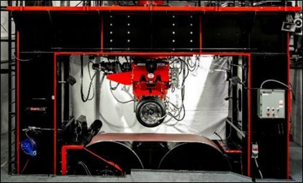
Figure 1. Calspan tire test machine, sourced from [1]
Calspan’s tire testing machine is capable of controlling a vast array of operating parameters as necessary to reproduce real-world operating conditions as closely as possible; those relevant to the TTC are shown below in Table 1.
Table 1. Calspan tire testing machine capabilities notable to the TTC, adapted from [1].
|
Description |
Units (Metric) |
|
Units (Imperial) |
|
|
Maximum Vertical Load |
kN |
53 |
lbf |
12,000 |
|
Lateral Force Capability |
kN |
± 40 |
lbf |
8992 |
|
Longitudinal Force Capability |
kN |
± 40 |
lbf |
8992 |
|
Slip Angle Range |
deg |
± 30 |
deg |
± 30 |
|
Maximum Slip Angle Rate |
deg/s |
15 |
deg/s |
15 |
|
Inclination Angle Range |
deg |
± 25 |
deg |
± 25 |
|
Inclination Angle Rate |
deg/s |
7 |
deg/s |
7 |
|
Spindle Speed |
rpm |
± 3,600 |
rpm |
± 3,600 |
|
Spindle Torque at 850 rpm |
kNm |
10.8 |
lb-ft |
8000 |
|
Spindle Torque at 2200 rpm |
kNm |
6.9 |
lb-ft |
5110 |
|
Spindle Torque at 3600rpm |
kNm |
2 |
lb-ft |
1440 |
|
Spindle Torque Rate |
kNm/s |
19 |
lb-ft/s |
14,000 |
|
Disk Brake Torque |
kNm |
20 |
lb-ft |
14,000 |
|
Maximum Lateral Belt Travel |
mm |
±5 |
in |
0.2 |
Resulting experimental data, data derived from the experimental data, as well as ambient test conditions, is then collected and stored into a series of channels, which is then uploaded to the TTC. The number of channels and data collected is dependent on the test, the full list of data channels created for the TTC round 9 tests are as follows:
Table 2. Round 9 TTC test data output channels, retrieved from [2]
|
Channel |
Units |
Description |
|
AMBTMP |
degC or degF |
Ambient room temperature |
|
ET |
sec |
Elapsed time for the test |
|
FX |
N or lbf |
Longitudinal Force |
|
FY |
N or lbf |
Lateral Force |
|
FZ |
N or lbf |
Normal Load |
|
IA |
deg |
Inclination Angle (Camber) |
|
MX |
N-m or lb-ft |
Overturning Moment |
|
MZ |
N-m or lb-ft |
Aligning Torque |
|
N |
rpm |
Wheel rotational speed |
|
NFX |
Dimensionless |
Normalized longitudinal force (FX/FZ) |
|
NFY |
Dimensionless |
Normalized lateral force (FY/FZ) |
|
P |
kPa or psig |
Tire pressure |
|
RE |
cm or in |
Effective Radius |
|
RL |
cm or in |
Loaded Radius |
|
RST |
degC or degF |
Road surface temperature |
|
SA |
deg |
Slip Angle |
|
SL |
Dimensionless |
Slip Ratio based on RE (such that SL=0 gives FX=0). This is “traditional” or “textbook” slip ratio. |
|
SR |
Dimensionless |
Slip Ratio based on RL (used for Calspan machine control, SR=0 does not give FX=0) |
|
TSTC |
degC or degF |
Tire Surface Temperature–Center |
|
TSTI |
degC or degF |
Tire Surface Temperature–Inboard |
|
TSTO |
degC or degF |
Tire Surface Temperature–Outboard |
|
V |
kph or mph |
Road Speed |
All data is reported in the SAE coordinate system as defined by SAE J2047 as shown below in Figure 2.
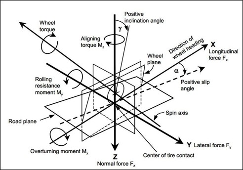
Figure 2. SAE tire sign convention, retrieved from [3]
Notable implications resulting from the SAE tire coordinate system revolve around how the relationship between longitudinal force (Fx) vs slip ratio (κ/SR/SL), lateral force (Fy) vs slip angle (α/SA), overturning moment (Mx) vs slip angle, and rolling resistance (My) vs slip angle are influenced. A positive slip angle, facilitated by a wheel rotation about the -Z axis, will produce a negative lateral force and will create an overturning moment and aligning moment about the +X axis (provided the slip angle does not exceed peak Mz production). These forces and moments are further influenced by the addition of inclination angle (camber) (γ), as depicted below in Figure 3, retrieved from [4]. Figure 3 invokes the following conditions: Fz < 0, My > 0.
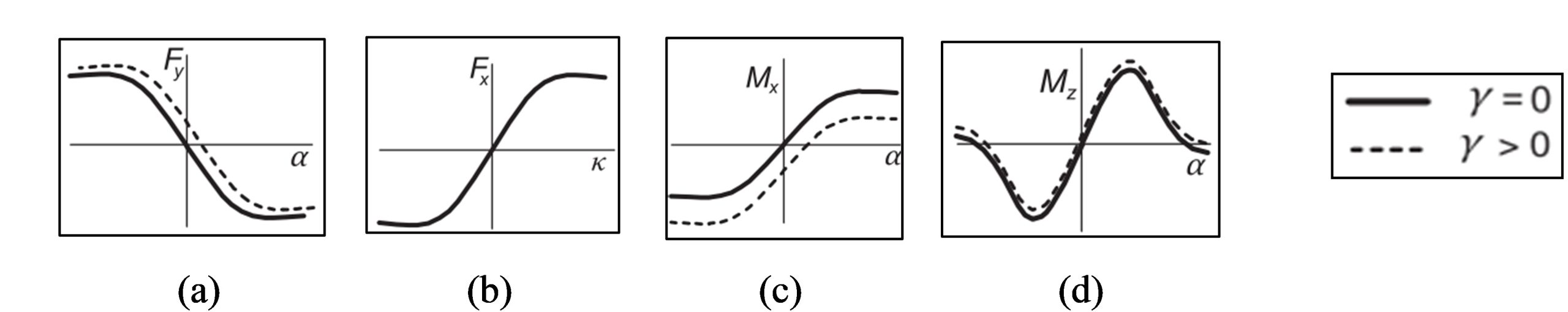
Figure 3. (a) longitudinal force vs slip ratio, (b) lateral force vs slip angle, (c) overturning moment vs slip angle, (d) aligning moment vs slip angle.
2.3. Calspan Tire Test Procedures
For the round 9 test, the following tires were tested, each on two different rim widths, the specific wheel and tire specifications to be used in this year’s model are highlighted in green.
Table 3. Round 9 wheel/tire test combinations.
|
Tire Manufacturer |
Size: O.D. x width x I.D. (in) |
Compound |
Wheel Size (in) |
|
Hoosier |
16.0×6.0-10 |
R20, C2000 |
10 x 6 |
|
Hoosier |
16.0×6.0-10 |
R20, C2000 |
10 x 7 |
|
Hoosier |
16.0×7.5-10 |
R20, C2000 |
10 x 7 |
|
Hoosier |
16.0×7.5-10 |
R20, C2000 |
10 x 8 |
|
Hoosier |
18.0×6.0-10 |
R20 |
10 x 6 |
|
Hoosier |
18.0×6.0-10 |
R20 |
10 x 7 |
|
Hoosier |
20.5×7.0-13 |
R20 |
13 x 7 |
|
Hoosier |
20.5×7.0-13 |
R20 |
13 x 8 |
|
MRF |
18.0×6.0-10 |
ZTD1 |
10 x 6 |
|
MRF |
18.0×6.0-10 |
ZTD1 |
10 x 7 |
|
Goodyear |
18.0×6.5-10 |
Eagle Racing Special |
10 x 6 |
|
Goodyear |
18.0×6.5-10 |
Eagle Racing Special |
10 x 7 |
|
Goodyear |
20.0×7.0-13 |
Eagle Sports Car Special |
13 x 7 |
|
Goodyear |
20.0×7.0-13 |
Eagle Sports Car Special |
13 x 8 |
All 10-inch tires were tested on aluminum wheels from Keizer Aluminum Wheels, all 13-inch tires were tested on steel wheels from Diamond Racing Wheels [2]. For each wheel/tire combination, three tests were conducted: a low-speed transient test, a cornering test, a drive/brake test. Each test is outlined below.
2.3.1. Transient Test Plan
The test begins with a set of cold, non-rolling spring rate tests, followed by a set of cold, rolling spring rate tests. After the initial tests are completed, several low-speed transient tests are performed wherein the tire is stopped, steered to a new slip angle, and then rolled forward slowly. During the low-speed transient tests, steer angles of -1, +1, and +6 deg are used, returning to 0 deg in between each step steer input. These tests occur at 3 different vertical loads and tire pressures at 10, 12, and 14psig. Transient- test conditions are depicted below in Figure 4.
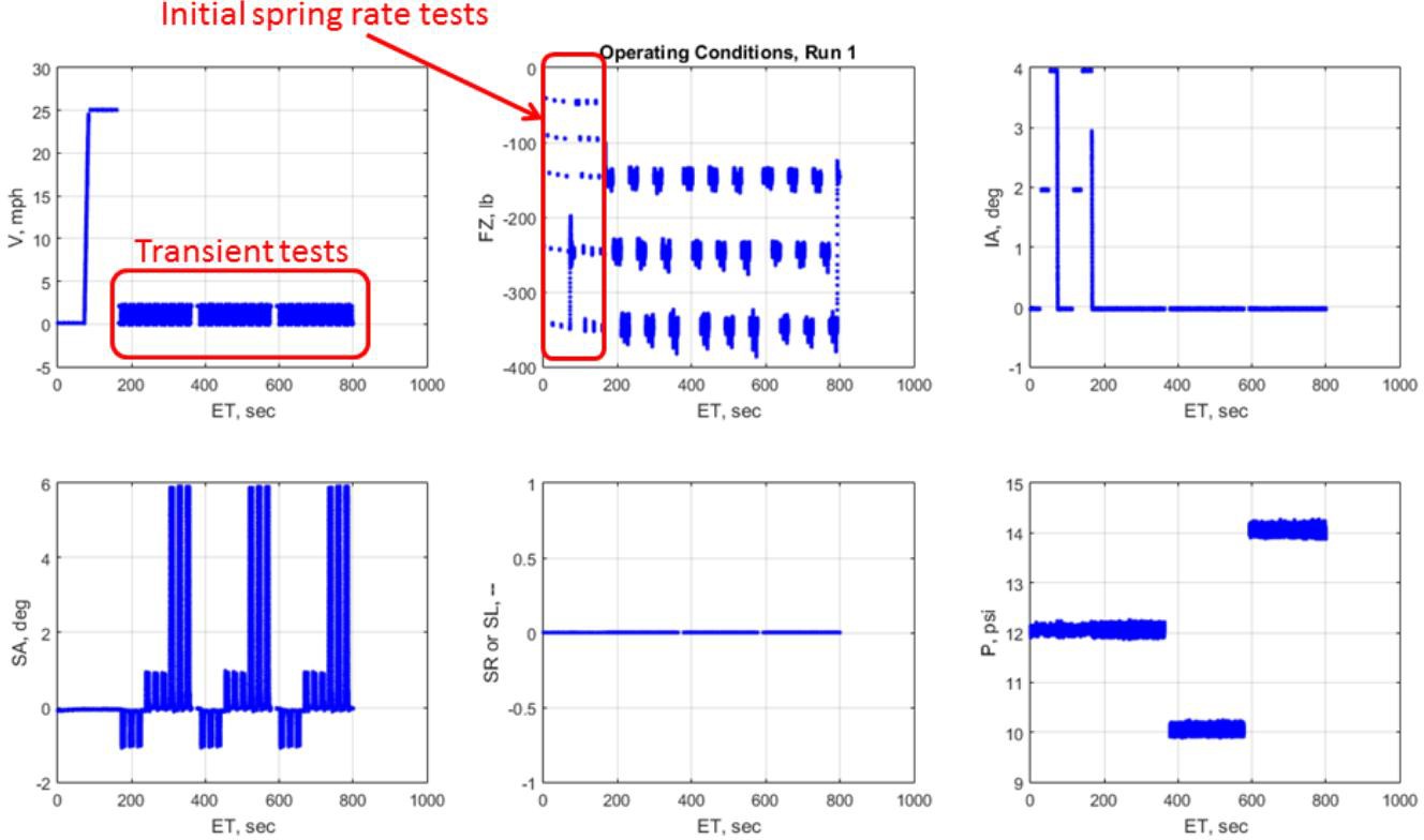
Figure 4. Transient test plan, reproduced from [2]
As the tire rolls slowly forward during the transient tests, it will seek a new equilibrium condition, the response distance required to reach an equilibrium condition is commonly referred to as “relaxation length”. The relaxation length metric is used as an indication of a tire’s transient response and is further characterized by the plots below, sourced from [2].
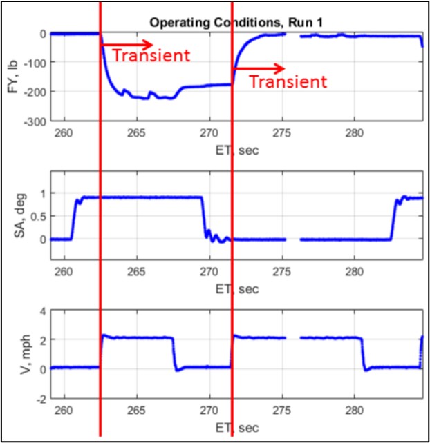
Figure 5. Transient tire characteristics for one steer out, steer back cycle
2.3.2 Cornering Test Plan
Initially, tires undergo a series of 12 “cold to hot” slip angle sweeps at a single load to condition them for accurate force and moment measurements while also evaluating the tire’s performance as it heats up. The test included multiple spring-rate assessments, starting right after the preliminary sweeps. Then subsequent tests were conducted at the end of each pressure segment.
Following a “break-in block” to further exercise the tire, the main slip-angle sweeps cycle through ±12 degrees at varying loads, pressures, and inclination angles, with the first slip angle sweep block being longer than the rest as a result of a few initial “conditioning sweeps”. All tests were conducted with zero slip ratio to maintain a free-rolling state. The first half of the test, shown below in Figure 6, covered three pressure levels, followed by a pause for data collection.
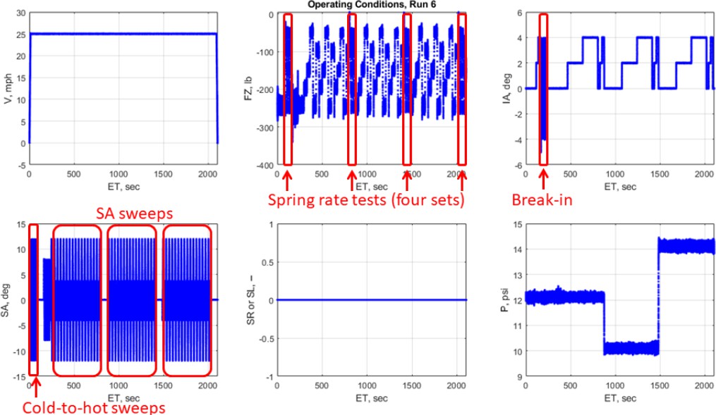
Figure 6. First half of the cornering test plan, retrieved from [2]
The second half resumes with another “cold to hot” block, mirroring the initial conditions of the test to restore the thermal state of the tire used in the first half of the test. Slip angle sweeps at 15 and 45 mph are conducted, run at zero inclination angle and 12psig. Finally, ± 4-degree inclination-angle sweeps at zero slip angle are run at all inflation pressures and three normal loads. The second half cornering test plan conditions are shown below in Figure 7.
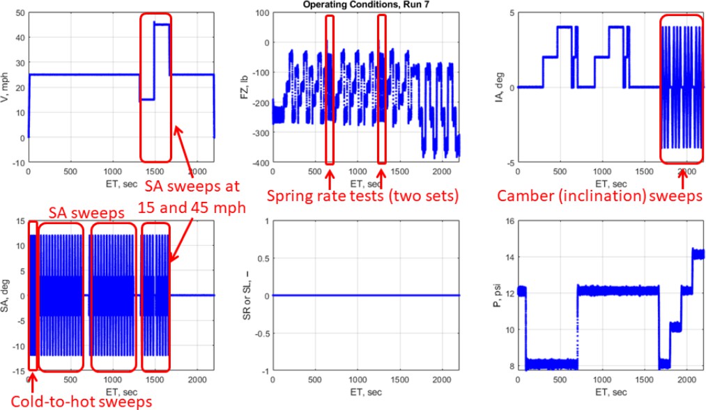
Figure 7. Second half of the cornering test plan, retrieved from [2]
2.3.3 Drive/Brake Test Plan
The drive/brake tests focus on slip ratio sweeps with constant slip angles. The tests begin with a warm- up that consists of three sets of spring rate tests, cold-to-hot slip angle sweeps, followed by simultaneous slip angle and inclination angle “break-in” sweeps, concluded by a series of slip angle conditioning sweeps. All of which were conducted in a free-rolling state. Warm-up test procedures are shown below in Figure 8.
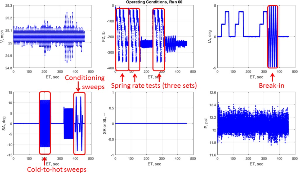
Figure 8 . Drive/Brake test warmup run plan, sourced from [2]
The bulk of the testing is split into two parts for data-management purposes, with each part conducted over various tire-pressure blocks. The first data collection segment, depicted below in Figure 9, covered three tire-pressure blocks with slip ratio sweeps at fixed slip angles of 0, -2, and -4 degrees. Although the data suggests varying slip angles, only the aforementioned fixed angles were actively used, with transitions between them captured within the sweeps.
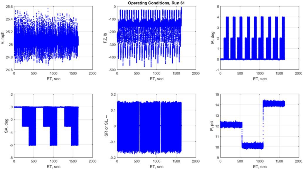
Figure 9. Drive/Brake test plan, first half, sourced from [2]
The test’s second half, shown below in Figure 10, includes an identical test procedure to the first half, conducted over an 8 and 12 psig tire pressure blocks. The test concludes with 15 and 45 mph slip-angle sweeps.
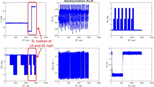
Figure 10. Drive/Brake test plan, second half, sourced from [2]
2.4. Aligning Tire Modeling Objectives with Test Data
Considering this is the inaugural attempt to construct a tire model, it is crucial to maintain simplicity in the modeling approach, allowing for reduced complexity in identifying areas for refinement.
Given the absence of past vehicle specifications and data, the ability to take advantage of previous vehicle data to produce “starting points” for suspension design and analysis was deemed unfeasible. Consequently, transient vehicle-response characteristics are excluded from consideration due to the lack of requisite known vehicle specifications, as the amount of input variables needed to produce a proper transient analysis far exceed what is known, can be estimated, or measured. Thus, transient tire data (refer to 2.3.1) is deemed superfluous, streamlining the model’s data requirements.
Steady-state analysis for cornering and acceleration offers a more manageable avenue, relying on conventional tire behavior metrics such as the relationship between lateral force and slip angle, and longitudinal force and slip ratio. The cornering test (refer to 2.3.2) and drive/brake test (refer to 2.3.3) have yielded extensive data across various operational conditions, such as inclination angle, pressure, and normal load that can be used in a steady-state vehicle analysis. Therefore, the tire model will be developed using data exclusively from the cornering and drive/brake tests.
3. Tire Modeling Overview and Model Selection
3.1. Tire Modeling Introduction
A tire model is a mathematical model of the tire that illustrates the behavior of a tire under various operating conditions. Tire models seek to predict the forces and moments generated by a tire as it interacts with the road surface, taking into consideration factors such as inclination angle, load, inflation pressure, temperature, and velocity.
Being the subject of extensive research, there are numerous tire models that exist, each aiming to reach a specific compromise between accuracy and complexity. Tire models typically fall under one of two categories; semi-empirical tire models – which describe tires using measured characteristics resulting from real-world testing and the usage of regression techniques to yield a best fit to the measured data, and theoretical tire models – which are aimed at a more detailed analysis of the tire albeit at the cost of introducing a large degree of complexity. Theoretical models typically come in the form of finite element- or segment-based models. There are a multitude of models that fall between semi-empirical and theoretical. The figure below, adapted from [4], provides further detail regarding tire model types.
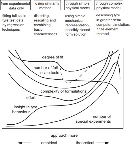
Figure 11. Various tire model types
3.2. Selecting a Tire Model
Considering the vast amounts of real-world test data produced by Calspan, it is evident that a semi- empirical tire model is necessary. This decision is further upheld considering the team’s high degree of inexperience with tire modeling at the time. Understanding and interpreting the results from a regression technique, such as mean squared error, are relatively easily understood when compared to analysis that might be required for a more theoretical model, such as RMOD-K.
Of all the semi-empirical tire models, the ‘Magic Formula’ tire model [4], created by Hans Pacejka, is by far one of the most widely used in industry. For the inaugural tire model, the Magic Formula will be used.
3.2.1. The Magic Formula Tire Model
The Magic Formula tire model is used to empirically represent and interpolate steady-state tire force and moment curves based on measured data. The coefficients within the formula act as representative quantities indicative of the tire’s performance attributes. The general form of the magic formula is given as
𝑌(𝑋) = 𝐷 𝑠𝑖𝑛[𝐶 𝑎𝑟𝑐𝑡𝑎𝑛{ 𝐵𝑥 − 𝐸(𝐵𝑥 − 𝑎𝑟𝑐𝑡𝑎𝑛 𝐵𝑥)}]
where
𝑌(𝑋) = 𝑦(𝑥) + 𝑆𝑣
𝑥 = 𝑋 + 𝑆ℎ
𝑆ℎ = horizontal shift
𝑆𝑣 = vertical shift
𝑆ℎ and 𝑆𝑣 arise due to the introduction of inclination angle or tire properties such as conicity or ply-steer and typically influence plots of lateral force and aligning moment [5].
𝑌 is either the lateral force (Fy), longitudinal force (Fx), or the aligning moment (Mz).
𝑋 is either the slip angle (α) or slip ratio (κ). Nomenclature for slip angle and slip ratio used in the TTC data channels, ‘SA’, ‘SL’, and ‘SR’, are not used in the Magic Formula.
𝐷 is the peak value.
𝐶 is the shape factor. This controls the span in the x direction and is given by
[latex]C = 1 \pm \left( 1 - \frac{2}{\pi}\,\arcsin\!\left(\frac{y_s}{D}\right) \right)[/latex]
𝐵 is the stiffness factor, controlling the slope at the origin.
𝐸 is the curvature factor. This influences the curvature at the peak and the point Xm where the peak occurs. 𝐸 is given by
[latex]E = \frac{B_{x m} - \tan\!\left({\pi}/{2C}\right)} {B_{x m} - \arctan\!\left(B_{x m}\right)}[/latex]
The 𝑦𝑎 term introduces an asymptote bounding 𝑌 at large slip angles and is found using
𝑦𝑎 = 𝐷 sin(π𝐶/2)
Curves produced by the Magic Formula typically take the form of the plot found in Figure 12 (a). For comparison, TTC test data for a single operating condition is shown in Figure 12 (b). The difference in plot orientation arises due to the Adapted SAE sign convention being utilized in the diagram reproduced from [4] and the standard SAE sign convention being utilized in Calspan’s data channels.
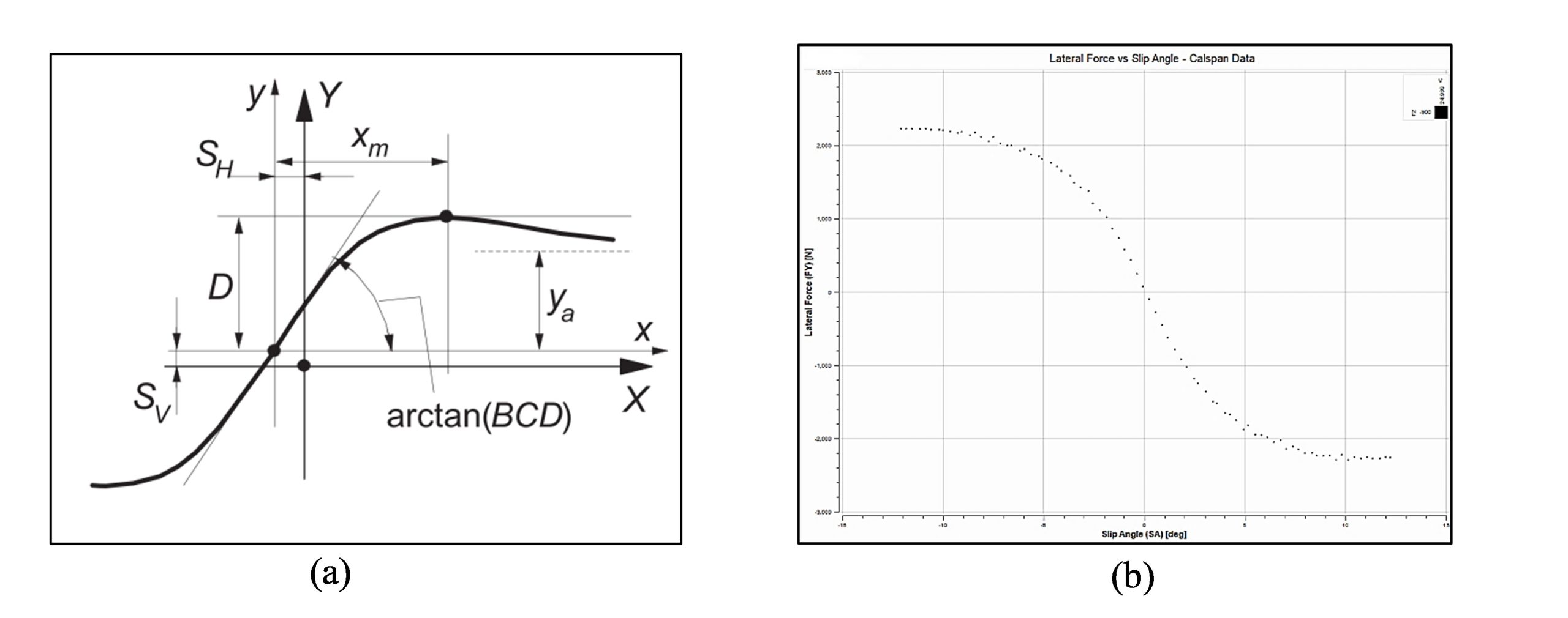
Figure 12 (a) Generalized tire model plot, (b) Calspan data
It must be noted that the complete list of equations and coefficients used within the Magic Formula are voluminous and extensive, full lists of these equations and coefficients can be found in [4] and [5].
4. Tire Model Development Procedure Using OptimumTire2
4.1. OptimumTire2 Introduction and Rationale for Selection
Developed by Optimum G, OptimumTire2 is a tire modeling software that specializes in generating tire models through the application of the Magic Formula to data derived from flat track tire testing, wherein models are created using a genetic algorithm regression model. The software is centered around a user- friendly interface and is complemented by continuously refined documentation. In-depth information on the full spectrum of OptimumTire2’s functionalities is elaborated in [6].
Given that OptimumTire2 is purpose-designed to generate Magic Formula tire models using datasets acquired from equipment akin to that employed by Calspan’s TIRF, its selection as the prime tool for this task is justified.
4.2. Importing and Processing Tire Data
TTC data is made available in a ‘raw’ and a ‘run’ format. Raw TTC data is made available for teams who want data with no pre-processing, meaning dwells between run sweeps are included. Run data has been pre-processed to remove dwells between run sweeps. This difference is shown below in Figure 13 for the FZ data channel.
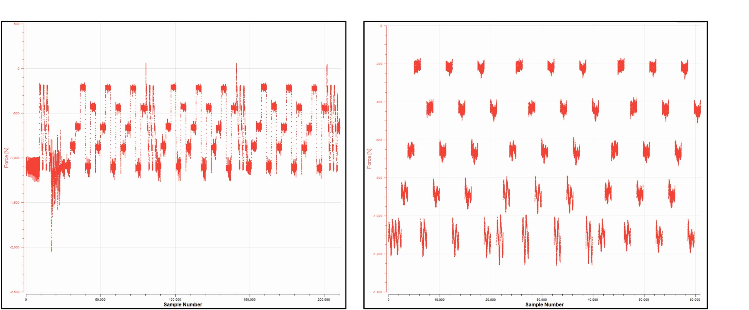
Figure 13. FZ raw data (left) compared to FZ run data (right), shown for the ‘Run31’ test dataset
While OptimumTire2 provides ample tools for manual data filtration and cropping, the decision was made to utilize only the run data as opposed to raw data. This decision was influenced by the potential for inadvertent error. Additionally, employing run data directly facilitates a smaller, more manageable dataset for the regression model, thus eliminating the need for identifying and rectifying fit errors.
Considering the decision made on tire data to be used in model development (refer to 2.4), the following data files shown in Table 4 were imported from the TTC into OptimumTire2. It must be noted that due to the warmup run file for the drive/brake test was omitted due to its extreme similarity to the warmup used in the cornering test.
Table 4. Test data used in tire model
|
Test |
Data File |
|
Cornering |
B2356run31 |
|
Cornering |
B2356run32 |
|
Drive/Brake |
B2356run72 |
|
Drive/Brake |
B2356run73 |
Although the run data represents a smaller, pre-processed form of the larger raw dataset as mentioned above, its volume remains relatively large, posing computational challenges for the genetic algorithm used by OptimumTire2. Specifically, extensive data risks excessive computational load, potentially leading to significant errors or hardware limitations. To mitigate this issue, a data pre-processing technique known as “binning” will be utilized. Data binning refers to the process of grouping a range of values into a smaller number of “bins”. Each bin represents a specific interval in the data range, allowing for a more streamlined and computationally efficient analysis while maintaining the integrity of the data patterns
OptimumTire2 allows for user-defined bin tolerances to be defined for each channel such that whenever the difference between the data value at index i+1 and the data value at index i is greater than the tolerance defined by the user for that specific channel, a new bin will be created [6]
4.2.1. Binning, Collapsing, and Merging Cornering Test Data
Recalling the cornering test plan as outlined in 2.3.2, the test primarily entailed variation of a single parameter, slip angle (SA), while holding fixed various operating parameters, such as normal load (FZ), pressure (P), or inclination angle (IA). In accordance with this methodology, each bin is defined to correspond to a distinct set of these operating conditions wherein every time FZ, P, or IA is changed, it is considered a new bin. Note that a specific bin tolerance will still be applied to the SA data channel to ensure each operating condition is binned with its respective slip angle sweep.
The two cornering datasets will eventually need to become one single dataset to perform the equation fit, this begs the question whether to bin and collapse data prior, or after the two datasets have been merged. Aiming to maintain simplicity within the data-binning process, the decision was made to bin and collapse each individual cornering datasets prior to merging them.
The criterion for determining the efficacy of the binning process will be based on the extent to which equal bin sizes can be achieved. This approach is rooted in the principle that uniformity in bin sizes is pivotal for ensuring a balanced and unbiased representation in the data analysis, thereby enhancing the accuracy of the equation fit.
Given the binning strategy and criterium stated above, the following binning tolerances shown in Table 5 were found to produce nearly equal bin sizes as shown in Figure 14 while simultaneously retaining trends found in the data as shown in Figure 15. Note that the binning tolerances given below in Table 5 were applied to both cornering test datasets.
Table 5. Binning tolerances for cornering test data
|
Data Channel |
Threshold |
Unit |
|
Normal Load (FZ) |
160 |
N |
|
Slip Angle |
10 |
deg |
|
Inclination Angle |
0.5 |
deg |
|
Pressure |
1 |
psi |
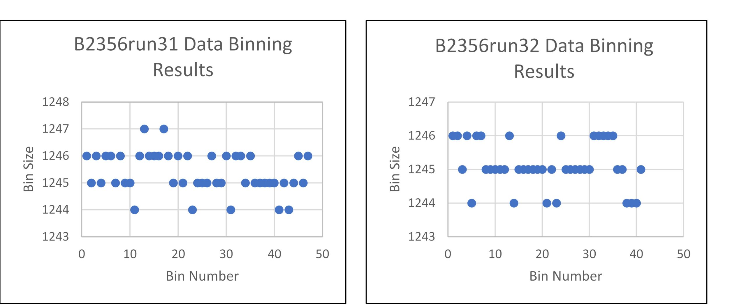
Figure 14. Cornering-test data-bin sizes
Following the data binning, the datasets will undergo a procedure known as “data collapsing”. Data collapsing is a method of summarizing multiple data points into a single representative value, typically by averaging nearby data points. Adhering to the default recommendation from OptimumTire2’s help guide [6], bin sizes will be reduced from those given in the binning results to 80 data points. The resulting data size after collapsing is shown below in Table 6.
Table 6. Cornering data collapsing results
|
Data File |
Data Size Before Collapsing |
Data Size After Collapsing |
|
B2356run31 |
61025 |
3760 |
|
B2356run32 |
52296 |
3280 |
A comparison between the unaltered run data and processed run data is shown below in Figure 15 for the normal load (FZ), inclination angle (IA), and pressure (P) data channels.
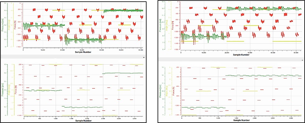
Figure 15. Collapsed cornering test data results sample for run 31 (left), run 32 (right)
With the two cornering datasets successfully binned and collapsed, they can be merged together into a single cornering dataset to be used in the equation fit procedure.
4.2.2. Binning, Collapsing, and Merging Drive/Brake Test Data
Similar to the approach outlined in 4.2.1, the binning of cornering data will also be structured around variations in testing parameters. FZ, IA, P, and SA, acting as the primary operating conditions as outlined in 2.3.3, will define the binning tolerances. As was done in 4.2.1, the SR channel will also act as a binning tolerance to ensure each operating condition is binned with its respective slip-ratio sweep.
Once again, data will be binned and collapsed prior to being merged together. The extent to which equal bin sizes can be achieved will remain as the measure of the quality of the binning process.
Following the binning procedure and evaluation strategy given above, bin tolerances for the drive/brake data could then be set. Unlike the cornering datasets, where bin tolerances could be found that yielded nearly identical bin sizes, extensive iterative testing was only able to yield bin sizes within 100 points of each other. This could be the result of several factors: the lack of “free rolling” with respect to slip angle that occurred during the drive/brake tests, larger datasets produced during the tests, and greater variability within the operating parameters are all possibilities that might have led to a discrepancy between bin sizes. A more decisive conclusion will require further research.
The binning tolerances given below in Table 7 produced the smallest difference between bin sizes for both drive/brake tests, bin sizes for each dataset are shown below in Figure 16.
Table 7. Binning tolerances for drive/brake test data
|
Data Channel |
Threshold |
Unit |
|
Normal Load (FZ) |
175 |
N |
|
Slip Angle |
0.5 |
deg |
|
Inclination Angle |
0.5 |
deg |
|
Pressure |
1 |
psi |
|
Slip ratio |
0.15 |
dimensionless |
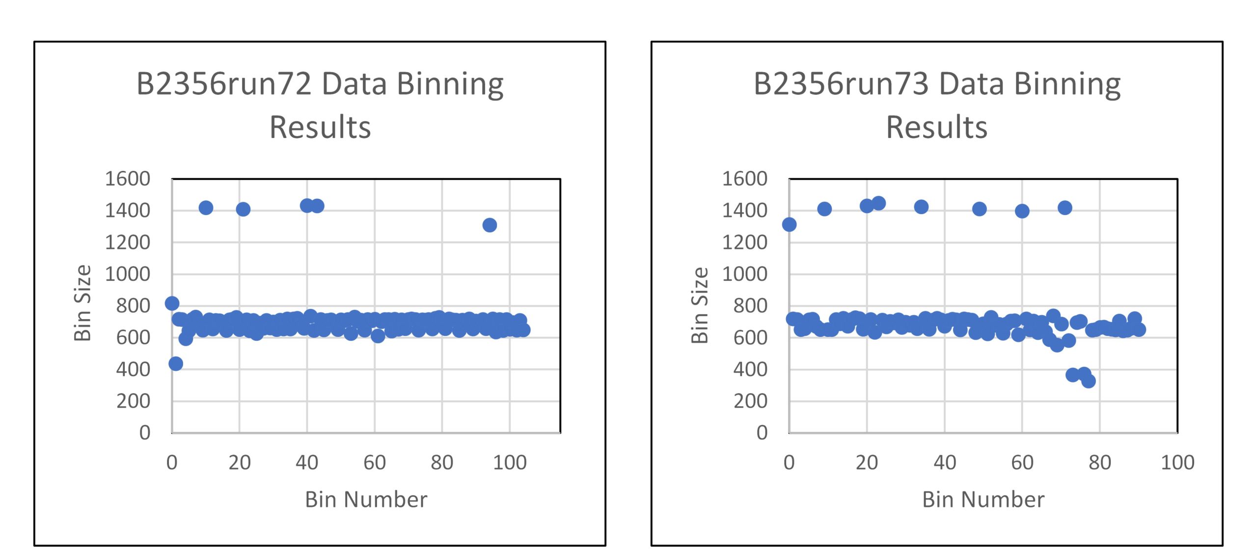
Figure 16. Drive/Brake test data bin sizes
Just as was done in 4.2.1, the datasets are to be collapsed in accordance with the default recommendation from OptimumTire2’s help guide [6]. The resulting data size after collapsing is shown below in Table 8.
Table 8. Drive/Brake data collapsing results
|
Data File |
Data Size Before Collapsing |
Data Size After Collapsing |
|
B2356run72 |
75860 |
8400 |
|
B2356run73 |
66778 |
7280 |
A comparison between the unaltered run data and processed run data is shown below in Figure 17 for the normal load (FZ), inclination angle (IA), and pressure (P) data channels.
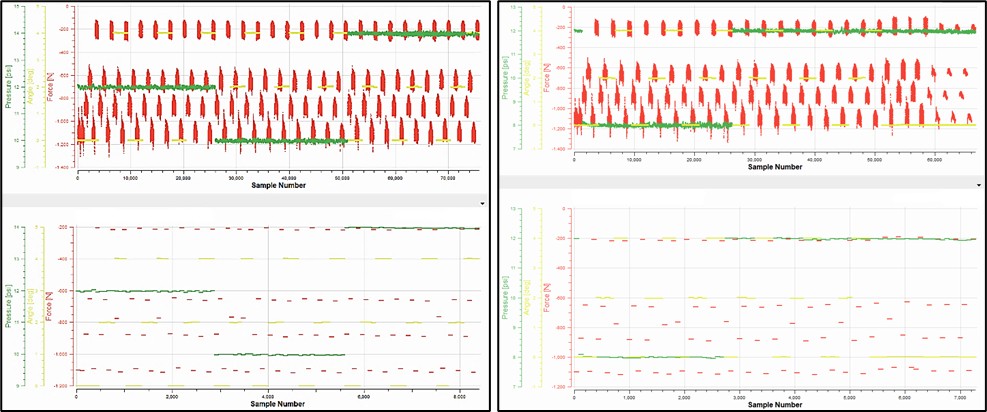
Figure 17. Collapsed drive/brake test data results sample for run 72 (left), run 73 (right)
The two datasets can now be merged into a single drive/brake dataset to be used in the equation fit procedure.
4.3 Magic Formula Equation-Fit Setup
4.3.1. Selecting the Magic Formula Version to be Used\
Due to its popularity, there are numerous versions of the Magic Formula that exist. Those available within OptimumTire2 are as follows:
- PAC2002 – This version of the Magic Formula is optimized for smooth road surfaces, accurately representing dynamic behavior for frequencies up to approximately 12 Hz. Unique to this version, it offers enhanced capabilities for interpolation and extrapolation beyond available measurement data.
- Magic Formula 5.2 – This version extends its modeling capabilities to include load sensitivity, lateral and longitudinal camber response, and effects of combined slips. Additionally, it accounts for rolling resistance and the tire’s overturning moment.
- Magic Formula 6.1.2 – This enhanced version of the MF-Tire 5.2 Magic Formula model features dynamic modeling that smoothly transitions from first-order relaxation to rigid ring dynamics. It also more accurately represents the impact of inflation pressure on loaded radius and tire enveloping properties, utilizing equations from the MFEval toolbox.
- Magic Formula 6.2 – This model enhances Magic Formula 6.1.2 by improving the loaded radius model for scenarios with large side slip and inclination angles. It includes tire load sensitivity, camber response, combined slip effects, and models both rolling resistance and tire overturning moment.
The selection of the appropriate Magic Formula version was guided by the principle of simplicity. OptimumTire2 offers a range of predefined boundary templates, which are instrumental in establishing the optimization constraints for the coefficients in the fitting process. Utilizing these templates significantly reduces the time investment required to individually define boundaries for each coefficient, thereby aligning with our objective of simplifying the analysis. As a result, the focus shifted to identifying the Magic Formula version for which these templates were readily available. Given the extensive availability of templates for the Magic Formula 6.1.2 model, it was determined that this version would be most suitable for fitting the data.
4.3.2. Setting Nominal Values
With the model version identified, the next step is to set the nominal inflation pressure (NOMPRES), nominal vertical load (FZNOM), and nominal longitudinal velocity (LONGVL). These are values that represent the ‘standard’ operating conditions for the tire. In light of the complete unavailability of test data, measurements, or calculations from preceding suspension systems, the selection of nominal values was predicated on their efficacy in yielding an accurate equation fit over a diverse spectrum of vertical load and inflation pressure conditions since these parameters are subject to significant variations. Following several meetings with the Optimum G engineers, the nominal values deemed to produce high fit accuracy across a wide range of data were found to be a nominal pressure of 82.7 kPa (12 psi), a nominal vertical load of -880 Newtons, and a longitudinal velocity of 11.163 meters per second.
4.3.3. Model Error-Calculation Method
Given the utilization of a predefined set of boundaries, as detailed in section 4.3.1, coupled with the intent to use a pre-optimized fitting algorithm, both of which are innate features of the software, it is logical to adopt the default error-calculation method provided. The default error-calculation method offered by OptimumTire2 that will be adopted for this year’s model is the root mean square deviation (RMSD). RMSD is a means of calculating the difference between an observed variable and a predicted variable, given as:
[latex]\text{RMSD} = \sqrt{\,\frac{1}{n}\,\sum_{i=1}^{n}\!\left(\text{predicted}_{i}-\text{observed}_{i}\right)^{2}}[/latex]
where 𝑛 represents the total number of observations and 𝑖 denotes the 𝑖th value within the dataset. RMSD results are interpreted as the magnitude of the prediction error. Within the context of empirical tire models, RMSD values represent the magnitude of error to which the model can accurately represent observed tire data.
With a model error calculation method chosen, all tire model properties necessary to perform an equation fit have been defined, they have been compiled and listed below in Table 9 for convenience.
Table 9. Tire model properties
|
Model Property |
Value |
Units |
|
Model type |
Magic Formula 6.1.2 |
N/A |
|
NOMPRES |
82737.1 |
Pascal |
|
FZNOM |
-880 |
Newton |
|
LONGVL |
11.163 |
Meters per second |
|
Error calculation method |
RMSD |
Dimensionless |
4.4. Performing the Equation Fits
4.4.1. OptimumTire2 Equation Fitting Procedure Overview
The OptimumTire2 Fitting Wizard uses a genetic algorithm [6] to perform an equation fit. The process begins with a diverse set of potential solutions, which are then iteratively evaluated for their ability to accurately fit the data. Through a cycle of selection (choosing the best solutions), crossover (merging different solutions), and mutation (introducing minor random variables), the algorithm refines these solutions over successive generations. The process concludes once an optimal fit is achieved through verification with an error calculation method, such as RMSD, or other termination criteria are met. Throughout this fitting procedure, the Magic Formula coefficients are optimized, within a set boundary to produce a tire model that is representative of a set of tire data. Prior to running a fit, the Fitting Wizard requires the evaluation function, genetic algorithm type, and boundaries to be defined.
4.4.2. Initial Setup – Lateral
As stated in 2.3.2, the tests were conducted in a free rolling state, meaning that a lateral force-pure (FYP) evaluation function is best suited for this dataset as it is specifically designed to perform the lateral equation fit to free rolling data. A ‘precise’ genetic algorithm type was selected for use on the basis of device computational capabilities at the time. Boundaries, as mentioned in 4.3.1, were to come from the “MF612-Fyp-Boundaries” template provided by OptimumTire2.
4.4.3. Performing the Lateral-Equation Fit
Building upon the data processing techniques, tire model properties, and genetic algorithm settings elaborated in the above sections, the lateral equation-fitting job was executed. The results of the fitting procedure are discussed below.
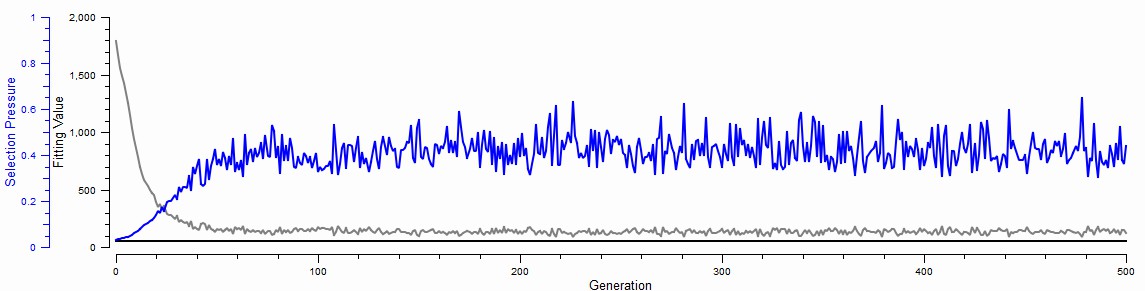
Figure 18. Genetic algorithm error plot for the FYP model fit
Figure 18, shown above, depicts the progression of the genetic algorithm up until its point of termination at iteration 500. The blue line denotes the selection pressure, this is the required fitness of the coefficients to the dataset to be selected for a particular generation. A selection pressure of 1 indicates the requirement for a perfect fit whereas a selection pressure of 0.1 would permit a broad spectrum of values to be eligible for selection. The grey line traces the RMSD, with convergence to the black baseline indicating a state of zero error, reflecting a perfect alignment between the model and the dataset.
Analyzing Figure 18, the genetic algorithm demonstrates a commendable performance in model fitting, indicated by a rapid initial decrease in RMSD, signifying a quick approach to a good fit. The subsequent stabilization and minor fluctuations in RMSD suggest that while the algorithm efficiently reduced the error, it did not achieve a perfect fit. Despite not reaching the ideal zero-error baseline, the algorithm succeeded in significantly improving the model’s accuracy.
4.4.4 Lateral-Fit Analysis
The genetic algorithm was able to fit the Magic Formula to the 7,040 cornering data points with an RMSD of 54.44. This suggests that while the overall fit captures the general trend of the tire behavior, certain regimes such as high slip angles may deviate from the experimental data, requiring specialized weighting functions if the model is to be further refined. Upon viewing the resulting tire model overlayed on the merged cornering data for various operating conditions such as normal load, pressure, and inclination angle as shown below in Figure 19, it is clear that the model captured the fundamental character of the data quite well.
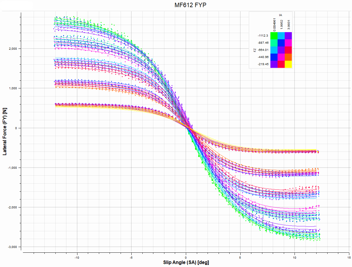
Figure 19. Lateral tire model overlayed on merged cornering data
While the resulting model is promising at first glance, further analysis is required to verify the model’s performance under various operating conditions, shown below in Figure 20.
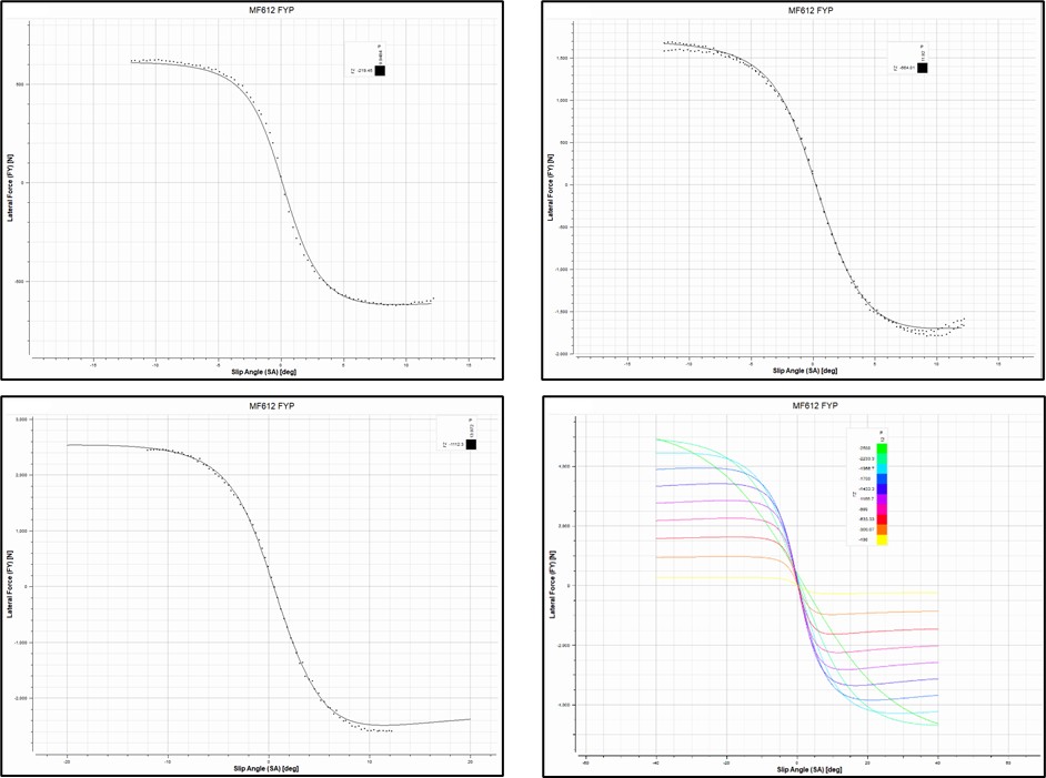
Figure 20 – FY vs SA at the following operating conditions:
Top left – 0 deg inclination angle, -219 N vertical load, 10 psi inflation pressure
Top right – 2 deg inclination angle, -664 N vertical load, 12 psi inflation pressure
Bottom left – 4 deg inclination angle, -1112 N vertical load, 14 psi inflation pressure
Bottom right – Vertical load from -100 N to -2500 N in increments of -266.67 N at a fixed inflation pressure of 12 psi and inclination angle of 1.5 degrees
Upon inspection of Figure 20, it is evident that the FY-pure tire model provides accurate representation of cornering tire data throughout a wide range of operating conditions. Observing the bottom right figure, it becomes clear that the extrapolative capacity of the model markedly diminishes at approximately – 2000 N of vertical load. This limitation, however, does not present a concern for Formula SAE applications, as the tires will not be subjected to such extreme loads during operation.
The analysis presented above leads to the conclusion that the lateral fit was successful. Consequently, the derived tire model establishes a sturdy foundation for analyzing the car’s dynamic response under a steady-state cornering maneuver.
4.4.5. Initial Setup – Longitudinal
Owing to the presence of combined slip conditions, characterized by concurrent slip angle and slip ratio during the drive/brake tests (refer to 2.3.3), the use of a ‘pure’ evaluation function was deemed unsuitable. Fortunately, OptimumTire2 incorporates an FX evaluation function, specifically designed to address instances of combined slip. For the longitudinal equation fitting, this FX evaluation function was selected. The “MF612-Fx-Boundaries” template was chosen as the boundaries for this equation fit.
4.4.6, Performing the Longitudinal Equation Fit
Leveraging the data processing techniques, tire model properties, and genetic algorithm settings elaborated in sections 4.2 through 4.4.5, the longitudinal equation fitting job was executed. The results of the fitting procedure are discussed below.
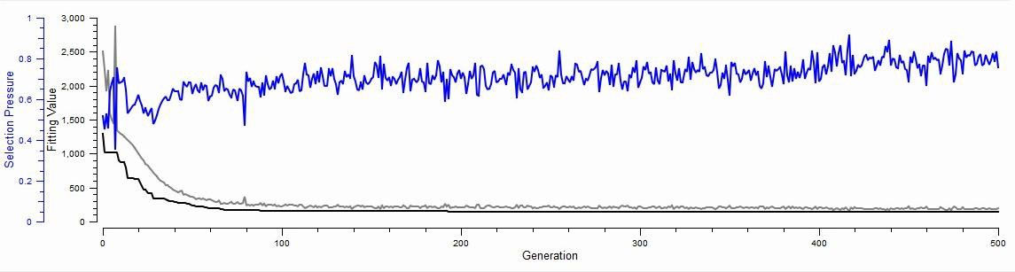
Figure 21. Genetic algorithm error plot for the FX model fit
Detail regarding the properties of each curve can be found in section 4.4.3. Upon inspecting the above error plot, the genetic algorithm exhibits a positive outcome in fitting the model. The initial sharp decline in the RMSD indicates a swift and significant improvement in fit accuracy. Over time, the RMSD levels off, suggesting the algorithm has reached a stable solution. Although the RMSD does not converge to zero, indicating the presence of some residual error, the overall trend shows the algorithm has effectively optimized the model parameters, striking a balance between fitting precision and computational efficiency over 500 generations.
4.4.7. Longitudinal-Fit Analysis
The genetic algorithm fit the Magic Formula to the 15,680 drive/brake data points with an RMSD of 147.861. This value indicates that, on average, the model’s outputs deviate from the measured values by 147.861 units. Although this RMSD is higher than that of the lateral fit, it is important to note that the drive/brake dataset includes an additional 8,640 points, which likely introduces extra variability and complexity into the fitting process. Moreover, when viewed relative to the overall range of measured data as shown in Figure 22, an average deviation of 147.861 units is within acceptable limits.
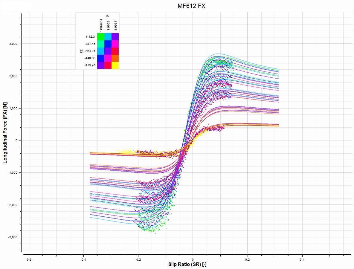
Figure 22. Longitudinal tire model overlayed on merged drive/brake data
As was done for the lateral fit, a more detailed analysis of the model’s resolution under specific operating conditions will be conducted, shown below in Figure 23.
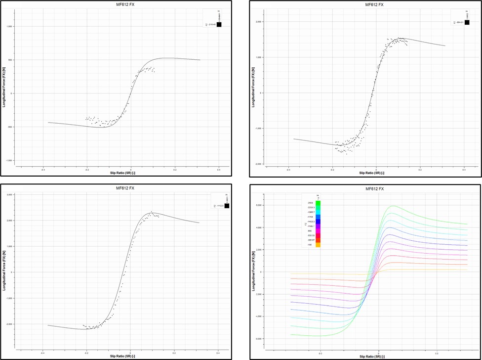
Figure 23. FX vs SR at the following operating conditions:
Top left – 0 deg inclination angle, -219 N vertical load, 10 psi inflation pressure
Top right – 2 deg inclination angle, -664 N vertical load, 12 psi inflation pressure
Bottom left – 4 deg inclination angle, -1112 N vertical load, 14 psi inflation pressure
Bottom right – Vertical load from -100 N to -2500 N in increments of -266.67 N at a fixed inflation pressure of 12 psi and inclination angle of 1.5 degrees
Upon examining the results, it is evident that the model exhibits a tendency to overestimate the longitudinal force response when subject to certain operating conditions. This overestimation is a probable factor contributing to the larger RMSD previously mentioned. A detailed investigation to pinpoint the exact operating conditions where this discrepancy occurs is presented in the following section.
4.4.7.1. Longitudinal-Force Response Error Analysis
Three distinct analyses were undertaken. In the first analysis, illustrated in the top left of Figure 24, the model parameters were set with a fixed vertical load (FZ) of -219.45 N and an Inclination Angle (IA) of 0 degrees, while varying the Pressure (P) at 9, 12, and 14 psi shown left to right. The second analysis, depicted in the top right of Figure 24, maintained a constant FZ of -219.45 N and P of 12 psi, but altered the IA at 0, 1.5, and 2.3 degrees shown left to right. The third analysis, presented at the bottom of Figure 24, fixed P at 12 psi and IA at 0 degrees, and adjusted FZ at three different levels: -219.45, -664.01, and -1112.3 N shown left to right.
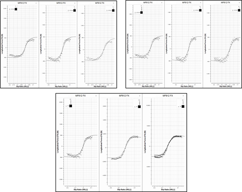
Figure 24. FX Response Patterns at Incremental Operating Parameters
By visual inspection, the following observations can be made:
- The influence of pressure on the model’s resolution is modest, with an improvement observed up to 12 psi. Beyond this threshold, a discernible reduction in resolution is apparent, particularly under positive slip ratios.
- Alterations in inclination angle seem to produce an insubstantial impact on the precision of the model.
- The most significant factor affecting the model’s resolution is the normal load. FZ values ranging from -600 N to -1200 N yield the most accurate alignment with the data.
From the above observations, it is likely that the considerable divergence from the -600 to -1200 N normal load range is likely responsible for the model’s deviation from the experimental data. This aligns with the nominal values established in section 4.3.2, which designated the nominal pressure at 82,737.1 Pascal (12 psi) and the nominal load at -880 N. Notably, departures from these nominal values appear to impact the model’s resolution more significantly than in the lateral model. This could be attributed to the larger amount of data making errors more pronounced or longitudinal-test conditions favoring low loads near a 12 psi inflation pressure. This heightened sensitivity could be due to the larger dataset amplifying discrepancies or because longitudinal testing conditions spent a larger time interval at low loads with pressures close to 12 psi.
The observed discrepancy In the ti”e mo’el has specific implications for suspension design, notably in areas dependent on the tire’s longitudinal characteristics such as acceleration, braking, and pitch behavior. These characteristics are sensitive to model inaccuracies, potentially leading to increased error in their analysis. However, such evaluations often focus on the more heavily loaded sections of the vehicle—for instance, the rear axle during acceleration—meaning that the error does not uniformly impact all analyses. Nonetheless, for comprehensive assessments like braking efficiency and the calculation of the ideal brake force ratio (IBFR), which involve the vertical load on all tires during braking events, the model’s lower load condition errors must be carefully considered.
5. Conclusion and Future Perspectives
The completion of Formula U Racing’s first tire model marks a significant advancement towards modernizing suspension design practices. Despite its simplicity, the model demonstrates encouraging conformity with Calspan’s test data. Excluding a particular range of operating conditions affecting the longitudinal model, it serves as a reliable tool for evaluating different suspension architectures, offering substantial time and cost savings before the commencement of parts modeling, prototyping, or construction.
The model will serve as an essential tool in any steady-state analysis, particularly for examining the impact of different suspension configurations on tire force and moment response. This includes, for example, assessing how camber thrust influences the maximum sustainable lateral acceleration during constant-radius skidpad tests. Additionally, the model will be invaluable for its implicit tire properties that are not immediately apparent in the plots. These properties, like cornering stiffness, are crucial for evaluating key dynamics such as understeer gradient, critical speed, and characteristic speed in steady- state cornering scenarios. This comprehensive utility makes the model a significant asset in optimizing vehicle performance.
Future advancements in tire modeling at Formula U Racing will focus on adopting a more interactive approach towards tire data management, including personalized data cropping and filtration. Efforts will also be directed towards developing tailored coefficient boundaries and customizing the genetic algorithm within OptimumTire2. These modifications are targeted at reducing RMSD or optimizing whichever model error evaluation method is chosen. As the team gains proficiency and familiarity with tire modeling, the models will evolve to encompass more complexity. This will include the integration of transient data, applications of weighting functions for specific operational conditions, and exploration into alternative versions of the Magic Formula, such as MF6.2. As Formula U Racing ventures into the future of suspension design, it is an exciting and hopeful time, signaling a significant step forward in the team’s technical journey.
References
[1] from Calspan_Round9. Index page. (n.d.). https://www.fsaettc.org/
[2] RunGuide_Round9. Index page. (n.d.). https://www.fsaettc.org/
[3] Kasprzak, E. M., & Gentz, D. (2006). The formula SAE tire test consortium-tire testing and data handling. SAE Technical Paper Series. https://doi.org/10.4271/2006-01-3606
[4] Pacejka, H. B., & Besselink, I. (2012). Tire and Vehicle Dynamics. Elsevier.
[5] Blundell, M., & Harty, D. (2015). The multibody systems approach to vehicle dynamics. Butterworth-Heinemann
[6] Avi, A., & Serpa, B. (2023). OptimumTire2 Help. Wiki. https://optimumg.atlassian.net/wiki/external/483426322/M2JmNTgzY2NkOTJiNGM5OTgwZTM1NzNiM2IwZTVkMzM#Welcome
[7] Braden, D. P. (2019). Tire Analysis and Modeling For The Development of an FSAE Car.
[8] Root mean square error (RMSE). Kalman filter for professionals. (2022, September 25). https://kalman-filter.com/root-mean-square-error/
[9] FSAEOnline.com. (n.d.). Www.fsaeonline.com. https://www.fsaeonline.com/
[10] FORMULA STUDENT (FSAE). (2025). Hoosiertirewest.com. https://www.hoosiertirewest.com/categories/circuit-racing-road-course-rally/formula-student-fsae.html
[11] Calspan Aerospace, Defense, and Automotive Testing. (2024). Calspan.com. https://calspan.com/
[12] Milliken Research Associates, Inc. — FSAE Tire Test Consortium. (n.d.). https://www.millikenresearch.com/fsaettc.html/www.millikenresearch.com/fsaettc.html
Media Attributions
- Figure 1
- Figure 2
- Figure 3
- Figure 5
- Figure 12
- Figure 13
- Figure 14
- Figure 15
- Figure 16
- Figure 17
- Figure 20
- Figure 23
- Figure 24
