Faculty Mentor: Amy Lenz (Mechanical Engineering, University of Utah)

 

INTRODUCTION

Ankle osteoarthritis (AOA) occurs in approximately 1% of the adult population worldwide and creates lasting and debilitating mental and physical conditions for those with it [1]. As such, necessary measures need to be taken to alleviate potential sources of pain and decreases in mobility. This can be accomplished within the stages of diagnosis and onset prediction using computational analysis and imaging techniques.

Currently, there are two main techniques that can be used to diagnose AOA: radiography and raw cone-beam weight-bearing computed tomography (WBCT). Radiography is the most conventional technique used to image and diagnose ankle OA. However, this technique has many limitations, which include the radiation dose from multiple radiographs, increased error due to difficulty taking images in the correct orientations [2], and occlusion of bony morphology in the complex ankle anatomy [3].

WBCT has been established as an alternative approach that provides a more accurate and comprehensive view of the ankle complex in three dimensions (3D) [2]. Although this technique eliminates bony occlusion, it can be difficult to ascertain features through viewing the three orthogonal perspectives of a medical imaging viewer separately.

A new way WBCT data can be analyzed is by using statistical shape modeling (SSM), which is a tool that allows for the quantitative study of anatomical morphology and alignment [4]. One such tool is ShapeWorks, developed at the University of Utah Scientific and Imaging Institute (SCI), an open- source SSM software that uses particle-based modeling applied to 3D shape models [5]. ShapeWorks can allow clinicians to view alignment, morphology, and other skeletal structures from WBCT in 3D from one perspective. However, to use 3D analysis in clinics, shape models need to be synthesized from images quickly and reliably. Convolutional neural networks (CNNs), a class of deep learning models, are particularly useful for processing image data by automatically learning variability of features from input images. In comparison to manual processing, CNNs reduce the time necessary to create shape models from WBCT images while producing comparable results [6]. This work aims to build on the prior work to create a functional convolutional neural network that analyzes the tibiotalar joint to classify populations with tibiotalar osteoarthritis and healthy populations.

To apply convolutional neural networks, WBCT images and their corresponding shape models can be input into a ShapeWorks module called DeepSSM, where parameters can be tuned and optimized to improve the network. The network described will quickly and reliably generate 3D statistical shape models automatically from WBCT images. Through analysis of the foot and ankle using DeepSSM, the time needed for 3D shape model analysis can be decreased, making it more feasible in the clinic. Ultimately, this new quantitative method for osteoarthritis classification could decrease the time physicians spend on less complicated cases, enabling them to work more on documentation and other cases.

BACKGROUND

Ankle Osteoarthritis

Ankle osteoarthritis is characterized by a significant reduction in ankle mobility, changes in gait, and progressive joint pain, resulting in substantial physical and mental debilitation [3]. Not only is it debilitating, but AOA affects a much younger population than hip OA, particularly those with previous trauma to the ankle such as repeated ankle sprains, rotational ankle fractures, and previous ligament injuries [3]. These traumas commonly lead to tibiotalar osteoarthritis, a subtype of AOA that primarily affects the tibiotalar joint between the talus and tibia. The younger patient population increases the importance of mediating the deterioration of cartilage, since any total ankle replacements or other procedures would not function long enough within the body [3]. Given the nature of this disease, quality diagnostic techniques are important to best inform and assist physicians in deciding on a treatment.

Current Clinical Techniques

Published in 1957, the Kellgren and Lawrence system (KL Grade) is the current gold standard for OA diagnosis and classifies OA into five grades: “None, Doubtful, Minimal, Moderate, Severe” [7]. The KL Grade makes classifications based on two-dimensional radiographs, where bony occlusion can hinder diagnosis [3]. Using traditional radiographs can also increase the amount of radiation administered as radiographs must be taken in four positions to assess seven different angles, which are used as indicators of ankle alignment and other bony traits [2].

An alternative to radiography is cone-beam WBCT, which can image the effects of osteoarthritis in the ankle more accurately and provide more information by minimizing bony occlusion. The use of cone-beam WBCT allows clinicians and researchers to compute angles and other reference lines used in deformity assessments from landmarks within the leg, as opposed to the error- inducing method of manually calculating the axes within the ankle externally [8]. Although CT scans generally induce more radiation exposure than radiographs, collecting an appropriate series of radiographs increases the radiation emitted compared to cone-beam WBCT [2]. Additionally, bony occlusion does not impact WBCT since the images are three dimensional, and analysis can be accomplished with statistical shape modeling (SSM), which applies correspondence points onto the surface of 3D shapes and allows the points to redistribute under an energy optimization schema [4].

SSM is advantageous as it allows for quantitative study of anatomical morphology and alignment [4, 5]. This process is time intensive, however, and requires an understanding of the processing and optimization procedures causing the method to be impractical for physicians in its present form.

Deep Learning Approaches

To make this process more feasible, the application of machine learning in medical imaging has the potential to accelerate clinical workflows and quantitative analysis, particularly for shape analysis [6]. Machine learning, otherwise known as deep learning, can decrease human workload by training a computer algorithm to accomplish the same work. One type of deep learning model is convolutional neural networks (CNN), which are particularly useful for processing image data as they are composed of both pooling and convolutional layers that leverage the unique structure of image data. Pooling layers reduce the feature maps to better capture details such as shape and size, while the convolutional layers convolve the input with multiple kernels that extract pattern information [6], which creates a CNN that has its own prescribed number and order of layers. One such CNN is DeepSSM, an implementation of machine learning applied to SSM through ShapeWorks [5]. ShapeWorks is an open-source SSM software, developed at the Scientific and Imaging Institute (SCI), that allows for the quantitative study of anatomic morphology and alignment.

Beginning with WBCT images and ending with shape models, DeepSSM is an open-source software that applies CNNs to efficiently segment image data [5]. DeepSSM begins with preprocessing to optimize, groom, and align shape models produced from WBCT image data. Since training neural networks in image analysis requires an enormous amount of data, DeepSSM generates a synthetic data set with a much larger sample size based on the distribution of features in the initial data set [9]. Training in DeepSSM consists of two separate neural architectures named Base-DeepSSM and TL-DeepSSM. In Base-DeepSSM the WBCT images are processed through five convolution and pooling layers and three fully connected layers to produce the predicted principal component analysis loading shape descriptor [10]. TL-DeepSSM has two sections as well: the T and the L. The T section is identical to the Base-DeepSSM network except that the output is a latent vector instead of a shape descriptor. The L section is an autoencoder with both convolutional and deconvolutional layers and two fully connected layers [11]. Base-DeepSSM and TL-DeepSSM are trained on the same images and work in conjunction to predict the final shape model from WBCT and compare it to the provided shape model. DeepSSM tests the neural network by comparing the distances between corresponding points on the predicted and provided shape models for unseen data.

Knowing that ankle osteoarthritis (AOA) causes lifelong, debilitating mental and physical conditions [1] and that the disease affects a younger population than most degenerative joint diseases [3], an immediate, quantitative approach to diagnostics is necessary to best inform orthopaedic surgeons as they recommend therapies and surgical interventions. According to Chan et al., deep learning is a potential solution, given its ability to exceed clinician’s performance [12]. A common misconception, however, is that these tools will replace physicians [6]. On the contrary, a quantitative and computational technique such as deep learning allows physicians to spend more time on more complicated cases, surgeries, and appropriate reporting [6]. More specifically, DeepSSM can be applied to AOA to provide quick and accurate diagnostics on disease type and severity, which can reduce clinician workflow, enabling physicians to focus their time and energy on the more complicated treatments.

METHODS

This research aims to address the limitations in diagnosing and predicting the onset of AOA. Weight-bearing computed tomography (WBCT) offers a superior alternative to radiographs, enabling detailed three-dimensional (3D) analysis, yet its use is constrained by labor-intensive manual processes. To enhance the clinical applicability of WBCT, this study proposes leveraging statistical shape modeling through ShapeWorks (SCI Institute, Salt Lake City, UT). By integrating WBCT data into a CNN-powered pipeline, this project will streamline the classification of tibiotalar osteoarthritis, reducing processing time while maintaining accuracy. This approach aims to make advanced imaging techniques more practical in clinical settings, enabling faster and more reliable AOA diagnosis and management.

Pre-Processing

The WBCT (0.37 x 0.37 x 0.37 mm3 voxel) data for this project comes from 43 tali from patients diagnosed with tibiotalar osteoarthritis by a musculoskeletal radiologist and orthopaedic surgeon. Each talus was segmented semiautomatically with DISIOR version 2.0 (Bonelogic, Helsinki, Finland) and then manually segmented using Mimics version 24.0 (Materlialise, Leuven, Belgium).

The manual segmentation is to correct for errors in the semi-automatic segmentation. Next, the talus was groomed, smoothed, and decimated in 3-Matic (Materialise, Leuven, Belgium). Once this pipeline has been completed in all 43 tali, all data was imported into ShapeWorks 6.6.0-dev (SCI Institute, Salt Lake City, UT) to be further preprocessed. Within the Grooming Module of ShapeWorks, the left tali were reflected over the x-axis and aligned using iterative closest point alignment to ensure uniform laterality and a uniform axis for later comparison. Next, the Optimization Module was utilized to place 1024 discrete correspondence points on each talus. This module uses a method that relies on particle-based modeling where discrete correspondence points are placed on the surface of the 3D shapes. The points redistribute themselves under an energy optimization schema, presenting valuable information on the surface appearance and distinguishable features as the correspondence points on each talus can be compared.

Deep Learning

After the preprocessing steps, the data was applied to a deep learning algorithm within the DeepSSM Module of ShapeWorks. The DeepSSM Module has four stages: Prep, Augmentation, Training, and Testing. Once trained and tested, the DeepSSM Module can make the shape models from WBCT without the time-intensive manual work otherwise required. The Prep Stage was run with default settings to align the WBCT images as inputs and preprocessed shape models as outputs.

Additionally, a split was established between the 43 tali to ensure that 80% of the data was used for training and 20% was used for testing. Since deep learning requires an enormous amount of data, the Augmentation Stage learns the shape variation in the 43 tali and applied the same variation to 4000 tali to ensure there was enough training data. The Training Stage was run with a learning rate of 0.001 over 100 epochs. The accuracy of the training was calculated over each epoch using mean squared error between the manually segmented shape models and the shape models predicted by DeepSSM. Finally, the Testing Stage used the unseen testing data to validate the trained model. This validation testing inputted the WBCT image data into the model and compared the distance between the surfaces of the outputted shape model and the manually segmented shape model. A heat map of distance from the manually segmented shape model is generated on the outputted shape model.

To evaluate these results, the training set is analyzed to determine if the learning rate indicates convergence. Additionally, the locations of error on each testing talus are investigated and compared between the tali. The mean distances between the surfaces of the input and output tali are compared as well.

RESULTS

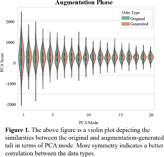
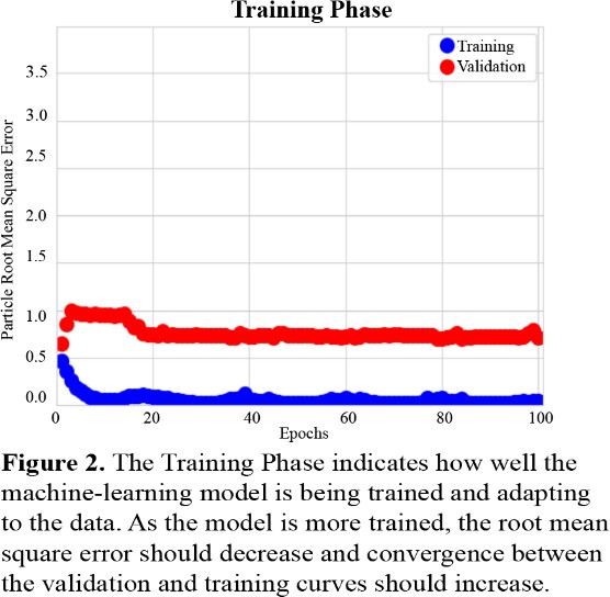
Figure 1 describes the relationship between the variability of the original 43 tali and the variability of the generated 4000 tali across 19 PCA modes. Each PCA mode is nearly mirrored between the original and generated data. The original data has a softer peak in many PCA modes in comparison to the generated data, indicating more variation and less of a normal distribution.

Figure 2 describes the success of the training phase. Training and Validation accuracies are plotted using root mean square error of the distance between discrete correspondence particles in the automatically segmented and manually segmented data. This is defined as the particle root mean square error as it is calculated on a particle-by-particle basis and averaged [5]. The errors remain low with all errors calculated to be below 1.0 throughout the training, however these errors do not converge to each other as expected. The validation error converges to a root mean square error of 0.75 and the training error converges to a root mean square error of near zero.

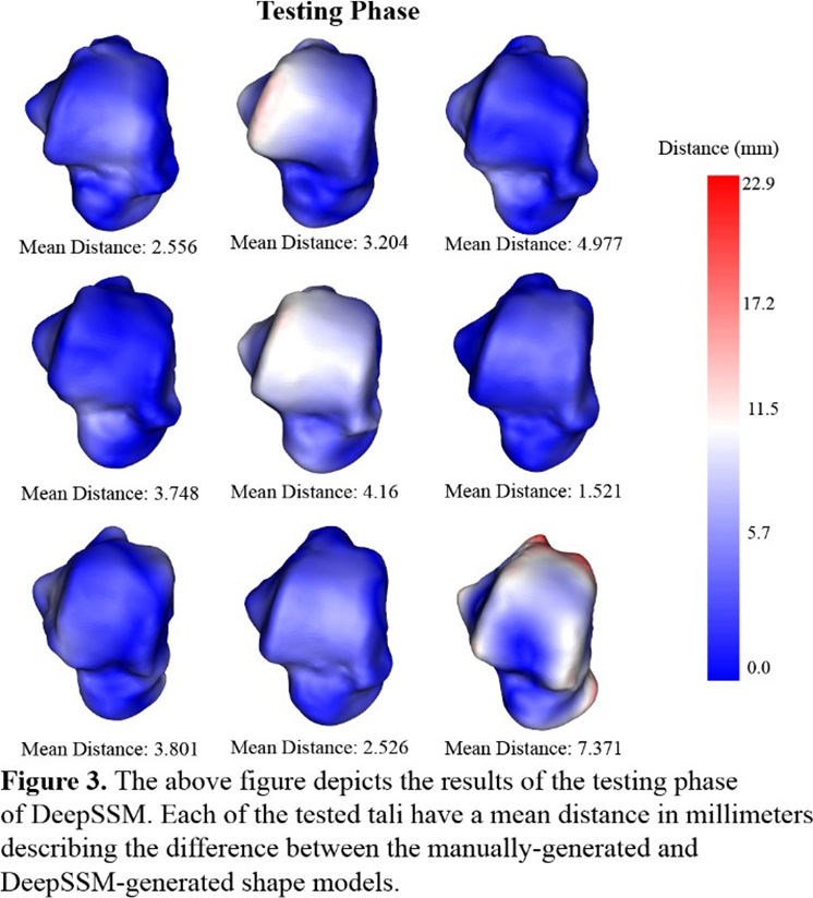
The third method of testing this neural network occurs in the testing phase. For each talus in the testing set, the discrete particles of the manually generated shape model are compared to the discrete particles of the automatically generated shape model by finding the distance between the corresponding particles. These 1024 distances are depicted on the talus using a heat map, with red indicating a larger distance and therefore more erroneous modeling. Additionally, the mean distance between corresponding particles is calculated for each of the tali in the testing set. Although most of the corresponding particles have low distances of near zero (indicated in dark blue in Figure 3) the model had larger distances (in red in Figure 3) on more patient-specific details. The center talus in the top row of Figure 3 depicts a protruding edge on the talar dome with large distances between the corresponding discrete points. Similarly, the bottom right talus has similar protrusions on the posterior process and the head correlating to large distances between the corresponding discrete points.

DISCUSSION

The goal of this study is to apply convolutional neural networks to generate 3D statistical shape models from WBCT images automatically. This involves utilizing a ShapeWorks module called DeepSSM, which enables the input of WBCT images and corresponding shape models, along with parameter tuning and optimization [5]. By integrating this approach into the analysis of the foot and ankle, the aim is to develop a method that decreases the time required for 3D shape model analysis, thereby increasing accessibility of such analyses in clinical settings. Ultimately, the long-term objective is to establish a quantitative framework for osteoarthritis classification that could improve efficiency in clinical workflows, allowing physicians to have more time to see more patients and complex cases.

In the results section, Figure 1 depicts that each PCA mode is nearly symmetrical, which indicates good correspondence between the initial 43 tali and the larger, augmented data set. This indicates that the data set that is later applied to the neural network model closely resembles the 43 tali in shape, size, and other variable traits. When the augmented data set is applied to training, Figure 2 describes low root mean square error, however the training and validation curves do not converge. This indicates that although the model is being trained and becoming more accurate, some parameters might need adjusting. The learning rate is likely slightly too high and might need to be decreased to allow for continued learning after the first few epochs. While Figure 2 depicts the model’s improvement over the course of training, Figure 3 demonstrates the model’s efficacy when used on unseen images. In this last phase, there are no epochs of learning and fixing mistakes, there is just one attempt to generate the shape model, and the generated shape model is compared to the manually made one. Figure 3 depicts that the model is fairly accurate at generating the new shape models, however certain regions were difficult for the model to generate accurately. This could have been for several reasons: the model was untrained on patient-specific morphology in that region, the tibiotalar joint is severely narrowed and there is bone-on-bone contact, or there is significant osteocyte growth in that region that was unseen previously by the model.

Several limitations should be acknowledged. The dataset size was limited to 43 tali, potentially reducing the model’s ability to generalize to broader populations. Additionally, the observed discrepancies in certain regions suggest that training data did not fully capture the morphological variability of AOA. Additionally, parameter tuning and optimization, including adjustments to the learning rate, could further improve model performance. Lastly, while the study demonstrates accuracy, real-world implementation would require extensive validation on larger, more diverse datasets. Future work can work towards decreasing these limitations through tuning and higher sample size.

This study aligns with recent advancements in applying machine learning to medical imaging, particularly in automating shape analysis and enhancing diagnostic workflows [5]. Existing literature supports the use of CNNs for pattern recognition and 3D reconstruction, yet the application to weight- bearing CT imaging for OA classification remains relatively underexplored [6]. By working to bridge this gap, the study contributes novel insights into leveraging automated shape analysis for specific clinical applications.

This work also has significant clinical implications. Enhanced imaging and automated analysis could facilitate earlier detection of AOA, enabling timely interventions to slow disease progression and improve long-term outcomes. Additionally, increased diagnostic efficiency has the potential to reduce healthcare costs by minimizing the need for manual processing, repetitive imaging, and delays. Faster and automated diagnostic tools would also enable clinicians to create patient-specific treatment plans and intervene before. deformities become too severe, ultimately improving care and outcomes for patients with AOA. Furthermore, efficiency in shape analysis could alleviate resource constraints in healthcare systems, particularly in underserved regions. By enabling quick detection, this work paves the way for improved patient care and outcomes on a global scale.

Reference

[1] M. Glazebrook et al., “Comparison of health-related quality of life between patients with end-stage ankle and hip arthrosis,” Journal of Bone and Joint Surgery, vol. 90, no. 3, pp. 499–505, 2008, doi: 10.2106/JBJS.F.01299.

[2] P. Kvarda et al., “3D Assessment in Posttraumatic Ankle Osteoarthritis,” Foot Ankle Int, vol. 42, no. 2, pp. 200–214, Feb. 2021, doi: 10.1177/1071100720961315.

[3] A. Barg et al., “Ankle osteoarthritis: Etiology, diagnostics, and classification,” Foot Ankle Clin, vol. 18, no. 3, pp. 411–426, 2013, doi: 10.1016/j.fcl.2013.06.001.

[4] J. Cates, S. Elhabian, and R. Whitaker, “ShapeWorks: Particle-Based Shape Correspondence and Visualization Software,” in Statistical Shape and Deformation Analysis: Methods, Implementation and Applications, Elsevier Inc., 2017, pp. 257–298. doi: 10.1016/B978-0-12-810493-4.00012-2.

[5] J. Cates, P. T. Fletcher, M. Styner, H. C. Hazlett, and R. Whitaker, “Particle-Based Shape Analysis of Multi-Object Complexes,” Med Image Comput Comput Assist Interv, vol. 11, no. 1, pp. 477–485, 2008.

[6] M. Kim et al., “Deep learning in medical imaging,” Dec. 01, 2019, Korean Spinal Neurosurgery Society. doi: 10.14245/ns.1938396.198.

[7] J. H. Kellgren and J. S. Lawrence, “RADIOLOGICAL ASSESSMENT OF OSTEO-ARTHROSIS,” Ann. Rheum. Dis., vol. 16, no. 4, pp. 494–502, 1957.

[8] M. Richter, C. de Cesar Netto, F. Lintz, A. Barg, A. Burssens, and S. Ellis, “The Assessment of Ankle Osteoarthritis with Weight-Bearing Computed Tomography,” Foot Ankle Clin, vol. 27, no. 1, pp. 13– 36, Mar. 2022, doi: 10.1016/j.fcl.2021.11.001.

[9] R. Bhalodia, S. Y. Elhabian, L. Kavan, and R. T. Whitaker, “DeepSSM: A Deep Learning Framework for Statistical Shape Modeling from Raw Images,” in Shape in Medical Imaging 2018 Lecture Notes in Computer Science, Springer International Publishing, 2018, pp. 244–257. doi: 10.1007/978-3-030- 04747-4_23.

[10] R. Bhalodia, S. Elhabian, J. Adams, W. Tao, L. Kavan, and R. Whitaker, “DeepSSM: A Blueprint for Image-to-Shape Deep Learning Models,” Oct. 2021, [Online]. Available: http://arxiv.org/abs/2110.07152

[11] R. Girdhar, D. F. Fouhey, M. Rodriguez, and A. Gupta, “Learning a Predictable and Generative Vector Representation for Objects,” Mar. 2016, [Online]. Available: http://arxiv.org/abs/1603.08637

[12] H. P. Chan, R. K. Samala, L. M. Hadjiiski, and C. Zhou, “Deep Learning in Medical Image Analysis,” in Advances in Experimental Medicine and Biology, vol. 1213, Springer, 2020, pp. 3–21. doi: 10.1007/978-3-030-33128-3_1.