Faculty Mentor: Andrej Cherkaev (Mathematics, University of Utah)

Abstract

The human body consists of highly complex and organized biochemical systems. There are count- less mechanisms at work that make the body function. In this study, we formulate a system of ordinary differential equations (ODEs) to model the concentration gradients of the various chemicals found in the Citric Acid cycle. The Citric Acid cycle, also known as the Krebs or TCA cycle, is the primary energy creation mechanism in the cell efficiently breaking down food sources into the necessary components for Adenosine Tri-phosphate (ATP) synthesis. The model considers the interactions of each of these chemicals, and the speed of the reactions, necessary to maintain a stable equilibrium. We assume a semi-closed system contained in the inner membrane of the mitochon- dria to simplify the model and reduce the number of variables. Using approximate steadystate concentrations for each chemical while at rest, we optimize the reaction rate constants such that the concentrations remain steady-state. This allows us to observe, mathematically, the aspects of the body that are used to govern the production of ATP in the body and maintain homeostasis.

Introduction

The Citric Acid cycle is a central mechanism in cellular respiration, playing a critical role in energy production by converting biochemical energy from nutrients into usable energy in the form of Adenosine Triphosphate (ATP). This series of enzymatic reactions occurs in the mitochondrial matrix. For a graphical representation of the Citric Acid cycle, see Appendix A.

Despite its complexity, the Citric Acid cycle operates with incredible consistency, maintaining a equilibrium among the concentrations of its intermediates and products. This equilibrium is essential for sustaining life, as disruptions in the cycle can lead to metabolic imbalances and cellular dysfunction. Understanding the underlying dynamics that govern this stability is therefore of significant interest.

In this project, we approach the Citric Acid cycle from a mathematical perspective. By constructing a system of ordinary differential equations (ODEs), which takes great inspiration from Bocharov et al., 2020 and pharmacokinetics, we aim to simulate the concentration gradients of the various chemicals within the cycle under the assumption of a semi-closed mitochondrial environment. That is, we have defined influx and outflux of certain metabolites and none for others, which is not necessarily the case in an applied setting. This is done for simplification as an open system would be too numerically complex and chaotic to be feasible mathematically.

Our objective is to identify reaction rate constants that result in a steady-state system, where the concentrations of the chemicals remain constant over time. This optimization problem not only shows the quantitative relationships necessary for metabolic stability but also highlights the utility of mathematical modeling in understanding complex biological systems. Through this study, we hope to provide a framework that deepens our insight into how the Citric Acid cycle works to maintains homeostasis and supports energy production.

Methods

The core of our system of ODEs to simulate the Citric Acid cycle is based around the kinetic reaction equation which is defined as:

dt
dx1 = k₀x₀ − k₁x₁(1)

where the change in the value of x₁ over the change in time t is equal to the rate at which x₁ is produced by the reaction k₀x₀, minus the rate at which x₁ is consumed by the reaction k₁x₁. For the system, we will assign each product in the cycle a variable as follows:

x₁ = Acetyl-CoA, x₂ = Citrate, x₃ = Isocitrate, x₄ = α–ketoglutarate, x₅ = Succinyl-CoA, x₆ =

Succinate, x₇ = Fumarate, x₈ = Malate, x₉ = Oxaloacetate, x₁₀ = NADH, x₁₁ = ATP.

There are also other substances produced and consumed by the system such as CO₂, H₂O, ADP, NAD+, HS-CoA enzymes, and other catalyzing enzymes, however, we will assume that these are in great enough abundance that their concentrations have a negligible effect on the core system itself and we will ignore these for the purposes of our model, establishing a semi-closed system.

The first step in the cycle is the introduction of Acetyl-CoA into the inner membrane of the mi- tochondria. This is achieved through various means such as pyruvate decarboxylation and beta- oxidation. For the purposes of our model, we simply combine all these methods and assign it a single rate constant variable k₀:

−→ Acetyl-CoA = k₀.(2)

Acetyl-CoA is then reacted with Oxaloacetate in the first step of the citric acid cycle to form Citrate and release an HS-CoA enzyme, which we represent as:

−→
Acetyl-CoA + Oxaloacetate ^k1 Citrate + HS-CoA

= k₁x₁x₉.(3)

Citrate reacts with a catalyzing enzyme and is reconstituted into Isocitrate and is represented as:

−→
Citrate ^k2 Isocitrate

= k₂x₂.(4)

Isocitrate is combined with an NAD+ molecule and produces CO₂, NADH, and α-ketoglutarate. NADH production will be accounted for in subsequent modeling steps. We will model this math- ematically as:

−→
Isocitrate + NAD+ ^k3 α–ketoglutarate + NADH + CO₂

= k₃x₃.(5)

α-ketoglutarate reacts with another NAD+ molecule and HS-CoA enzyme to produce NADH, CO₂, and Succinyl-CoA. Again, NADH production will be accounted for in subsequent steps and model this reaction with:

−→
α–ketoglutarate + HS-CoA + NAD+ ^k4 Succinyl-CoA + NADH + CO₂

= k₄x₄.(6)

Succinyl-CoA reacts with a GDP molecule and H₂O, releases the HS-CoA enzyme and produces GTP and Succinate. GTP is energetically equivalent so for the purposes of our model, it will be modeled as ATP. Like NADH, we’ll account for this in subsequent steps. This process is modeled as:

−→
Succinyl-CoA + H₂O + GDP ^k5 Succinate + GTP + HS-CoA

= k₅x₅.(7)

The Succinate then reacts with FAD and produces Fumarate and FADH₂. FADH₂ is similar enough to NADH that we will group them together and model them under one variable. We’ll ignore the FADH₂ for now and return to it later with the other NADH molecules. We’ll model this with:

−→
Succinate + FAD ^k6 Fumarate + FADH₂

= k₆x₆.(8)

Fumarate reacts with H₂O to become Malate:

−→
Fumarate + H₂O ^k7 Malate

= k₇x₇.(9)

We finally reach the end of the cycle to where Malate reacts with a NAD+ molecule to produce NADH and Oxaloacetate:

−→
Malate + NAD+ ^k8 Oxaloacetate + NADH

= k₈x₈(10)

where Oxaloacetate is once again consumed with Acetyl-CoA to start the cycle over again:

−→
Oxaloacetate ^k9

= k₉x₉.(11)

Now we can revisit NADH. Because NADH (and its equivalents) are a byproduct of the reactions in the Citric Acid cycle, it’s production is already modeled in the above equations, so the concen- tration of NADH is simply the product of those reactions which is modeled with the ODE 23 in our final system.

ATP is similar, however, it includes a reaction component as NADH is consumed to generate ATP which is modeled as:

−→
NADH ^k10 ATP

= k₁₀x₁₀.(12)

This is a gross oversimplification of oxidative phosphorylation, however, for the purposes of the model and showing the behaviors of the concentration gradients it is “good enough.” The con- sumption and transportation of ATP out of the mitochondria is similarly simplified with:

−→
ATP ^k11

= k₁₁x₁₁.(13)

The rational for this oversimplification being that since the body is so incredibly complex that, under the already existing assumptions such as operating in a closed system, this simplification is moot and the model provides a close enough approximation to provide the deeper understanding of how the Citric Acid cycle works that it primarily sets out to do.

With all variables and equations defined, we can assemble them into a system of ODEs, predicated upon equation 1:

dt
dx1 = k₀ − k₁x₁x₉(14)

dt
dx2 = k₁x₁x₉ − k₂x₂(15)

dt
dx3 = k₂x₂ − k₃x₃(16)

dt
dx4 = k₃x₃ − k₄x₄(17)

dt
dx5 = k₄x₄ − k₅x₅(18)

dt
dx6 = k₅x₅ − k₆x₆(19)

dt
dx7 = k₆x₆ − k₇x₇(20)

dt
dx8 = k₇x₇ − k₈x₈(21)

dt
dx9 = k₈x₈ − k₉x₉(22)

dt
dx10 = k₃x₃ + k₄x₄ + k₈x₈ − k₁₀x₁₀(23)

dt
dx11 = k₅x₅ + 5k₁₀x₁₀ − k₁₁x₁₁.(24)

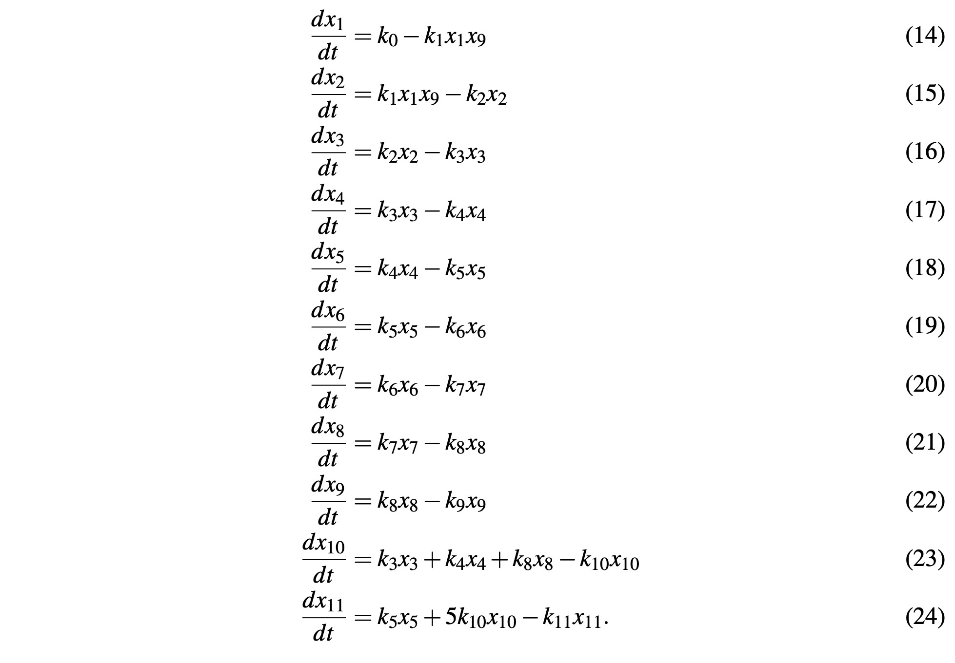
This is the final system of ODEs that will constitute our simulation for the Citric Acid cycle. Since our goal here is to identify the reaction rate constants k_i such that our system maintains equilibrium at steady-state concentrations of the variables x_i, we will define an optimization problem as:

11

min ∑ k_i(25)

k i=0

s.t. ∑ I dx I =
11

ⁱ0,

i=1 I dt I

k_i ≥ 0.001,∀i ∈ {0, 1, . . . , 11}.

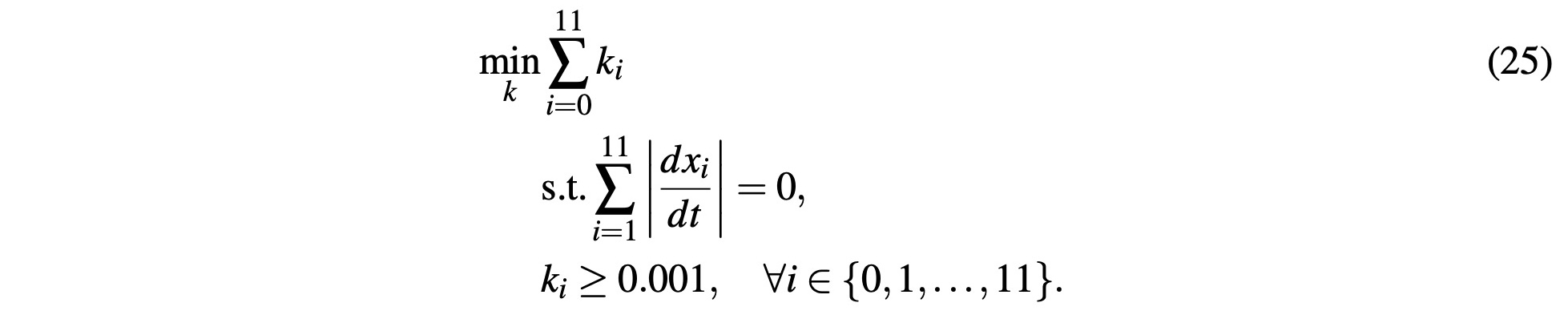
This ensures we get real, non-zero, values for k_i such that the derivatives of all equations are zero. We assume that the body strives to create the needed amount of ATP with the least exertion. Under this assumption, the optimization problem attempts to estimate the minimum reaction rates k_i so that it maintains constant concentrations of metabolites x_i. Using known and estimated values of metabolite concentrations in the body, solving and simulating the system revolves around this optimization problem.

Results

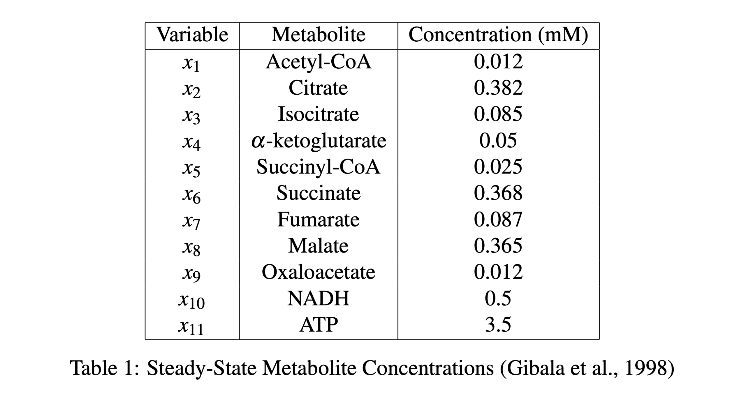
The model was simulated using Python. Using the following steady-state concentration values shown in table 1.

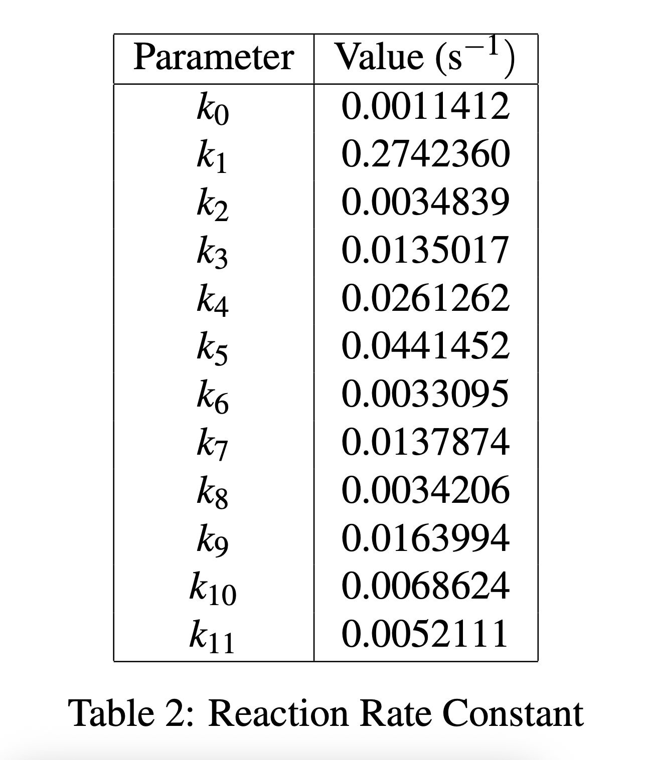
The system of ODEs is optimized using 25 and the kinetic reaction rate constants k_i are estimated as the values in table 2.

Running the simulation using the above k_i values and randomly generated initial concentrations x_i between [0, 1], we plot the change in concentrations over time and we get the following graph:

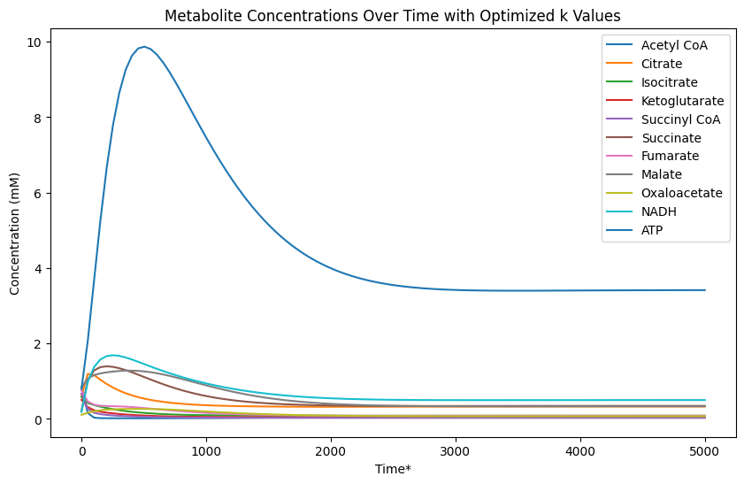
Figure 1: Concentrations

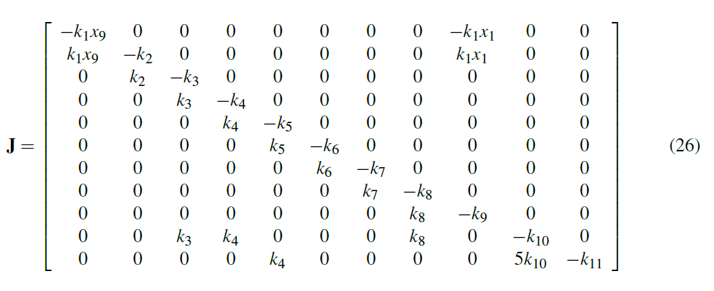
Here we observe a unique property of the system that no matter what concentration values we start with we always return to equilibrium at our steady-state concentrations in Table 1. To show this mathematically, and evaluate the stability of the system, we can compute the Jacobian matrix:

If we evaluate the Jacobian with the values in tables 1 and 2, and compute the eigenvalues, we get the following:

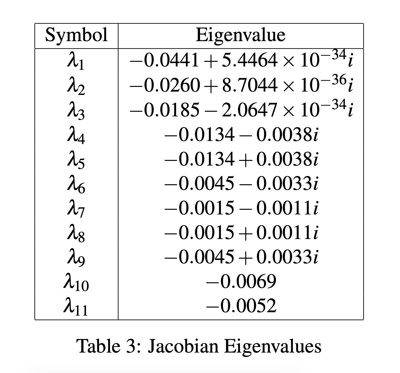
Table 3: Jacobian Eigenvalues

Because the real part of all the eigenvalues are negative, this shows that the system of ODEs is asymptotically stable and will always converge to an equilibrium point with the optimized k_i values.

Conclusion

Our results show that by optimizing reaction rate constants, the Citric Acid Cycle can be modeled as an asymptotically stable system, consistently returning to steady-state concentrations despite initial disturbances. This confirms the inherent optimization and stability of cellular metabolic regulation, even under simplified assumptions.

The steady-state optimization reflects the body’s biological preference for metabolic efficiency, suggesting that the availability and regulation of enzymatic catalysts may have evolved to achieve minimal energetic cost. This model may help explain how cells dynamically regulate energy pro- duction in response to demand.

This model necessarily simplifies a highly complex biochemical system. Factors such as feedback inhibition, transport of metabolites across mitochondrial membranes, and the role of oxygen and electron transport were not considered. These elements, while critical in reality, were excluded to focus on the cycle’s core dynamics and ensure feasibility.

Future work should be done, as more complex and realistic model could provide greater insight into how our bodies functions. With applications to general biology, medicine, kinesiology, sports science, and various other fields that study energy systems, this is an important area of study with unrealized benefits to science as a whole.

*The author acknowledges the support from NSF through RTG award (NSF DMS-2136198)

**ChatGPT was used as a tool to aid in the ideation and drafting of this paper. All content and ideas are the original creations of the author.

Bibliography

Alberts, B., Hopkin, K., Johnson, A., Morgan, D., Raff, M., Roberts, K., & Walter, P. (2019).Essential cell biology (5th). W. W. Norton & Company.

Bocharov, G., Jaeger, W., Knoch, J., Neuss-Radu, M., & Thiel, M. (2020). A mathematical model of hif-1 regulated cellular energy metabolism. Vietnam Journal of Mathematics, 49(1), 119–141. https://doi.org/10.1007/s10013-020-00426-y

Gibala, M. J., MacLean, D. A., Graham, T. E., & Saltin, B. (1998). Tricarboxylic acid cycle in- termediate pool size and estimated cycle flux in human muscle during exercise. AJP En- docrinology and Metabolism, 275(2), E235–E242. https://doi.org/10.1152/ajpendo.1998. 275.2.e235

Appendix A: Citric Acid Cycle Diagram

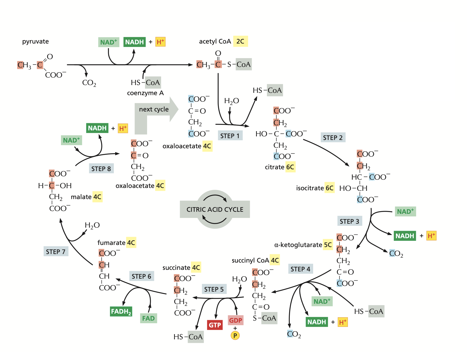
Figure 2: The Citric Acid cycle (Alberts et al., 2019)

Appendix B: Python Code

import numpy as np

import matplotlib . pyplot as plt

from scipy . integrate import solve_ivp from scipy . optimize import minimize import sympy as sp

import warnings warnings. filterwarnings(’ ignore ’)

# System of ODEs

def TCA_cycle_model (t, y, k):

Acetyl_Co A , Citrate , Isocitrate , Ketoglutarate , Succinyl_Co A ,

Succinate , Fumarate , Malate , Oxaloacetate , NADH , ATP = y

d Acetyl_Co A = ( k [0]) – ( k [1] * Acetyl_Co A * Oxaloacetate ) d Citrate = ( k [1] * Acetyl_Co A * Oxaloacetate ) – ( k [2] * Citrate ) d Isocitrate = ( k [2] * Citrate ) – ( k [3] * Isocitrate ) d Ketoglutarate = ( k [3] * Isocitrate ) – ( k [4] * Ketoglutarate ) d Succinyl_Co A = ( k [4] * Ketoglutarate ) – ( k [5] * Succinyl_Co A ) d Succinate = ( k [5] * Succinyl_Co A ) – ( k [6] * Succinate ) d Fumarate = ( k [6] * Succinate ) – ( k [7] * Fumarate )

d Malate = ( k [7] * Fumarate ) – ( k [8] * Malate ) d Oxaloacetate = ( k [8] * Malate ) – ( k [9] * Oxaloacetate )

d NADH = ( k [3] * Isocitrate ) + ( k [4] * Ketoglutarate ) + ( k [8] * Malate ) – ( k [10] * NADH )

dATP = ( k [4] * Succinyl_Co A ) + (5 * k [10] * NADH ) – ( k [11] * ATP )

return [ d Acetyl_Co A , dCitrate , d Isocitrate , d Ketoglutarate , d Succinyl_Co A , d Succinate , d Fumarate , dMalate , d Oxaloacetate , dNADH , dATP ]

# Rate constant optimization error function

def steady_state_error (k, y0 ):

sol = solve_ivp ( lambda t, y: TCA_cycle_model (t, y, k), (0 , 100) , y0 , t_eval =[100 ])

final_values = sol. y[:, -1]

derivatives = TCA_cycle_model (0 , final_values , k) return np. sum ( np. abs( derivatives))

# Rate constant optimization function

def optimize_k ( y0 ): initial_k = np. ones (12)

bounds = [(0.001 , 10) for _ in range (12)]

result = minimize ( lambda k: np. sum ( k), initial_k , bounds= bounds , constraints ={’ type ’: ’ eq ’, ’ fun ’: lambda k: steady_state_error ( k, y0 )})

return result. x

# Given initial conditions

constants = [0.012 , 0.362 , 0.085 , 0.05 , 0.025 , 0.368 , 0.087 , 0.365 ,

0.012 , 0.5 , 3.5]

optimal_k = optimize_k ( constants) print(’ Optimized k:’, optimal_k )

# Simulation space

t_span = (0 , 5000)

t_eval = np. linspace (* t_span , 100)

# Random initial values

y0 = np. random . rand (11)

# Solution to the system

solution = solve_ivp ( lambda t, y: TCA_cycle_model(t, y, optimal_k ), t_span , y0 , t_eval= t_eval)

# Plot the results

plt. figure ( figsize =(10 , 6))

metabolites = [’ Acetyl – CoA ’, ’ Citrate ’, ’ Isocitrate ’, ’ Ketoglutarate ’, ’ Succinyl – CoA ’, ’ Succinate ’, ’ Fumarate ’, ’ Malate ’, ’ Oxaloacetate ’, ’ NADH ’, ’ ATP ’]

for i, label in enumerate ( metabolites): plt. plot( solution .t, solution . y[ i], label= label)

plt. xlabel(’ Time *’) plt. ylabel(’ Concentration ( mM)’)

plt. title (’ Metabolite Concentrations Over Time with Optimized k Values ’)

plt. legend () plt. show ()

# Variables

x = sp. symbols(’ x1 x2 x3 x4 x5 x6 x7 x8 x9 x10 x11 ’) k = sp. symbols(’ k0 :12 ’)

# System of ODEs

dxdt = [

k [0] – k [1]* x [0]* x[8],

k [1]* x [0]* x[8] – k [2]* x[1],

k [2]* x[1] – k [3]* x[2],

k [3]* x[2] – k [4]* x[3],

k [4]* x[3] – k [5]* x[4],

k [5]* x[4] – k [6]* x[5],

k [6]* x[5] – k [7]* x[6],

k [7]* x[6] – k [8]* x[7],

k [8]* x[7] – k [9]* x[8],

k [3]* x[2] + k [4]* x[3] + k [8]* x[7] – k [10]* x[9],

k [4]* x[4] + 5* k [10]* x[9] – k [11]* x [10]

]

J = sp. Matrix ( dxdt). jacobian ( x) steady_state_values = {

x [0]: 0.012 , x [1]: 0.362 , x [2]: 0.085 , x [3]: 0.05 , x [4]: 0.025 , x [5]:

0.368 ,

x [6]: 0.087 , x [7]: 0.365 , x [8]: 0.012 , x [9]: 0.5 , x [10]: 3.5

}

parameter_values = {

k [0]: 0.0011412 , k [1]: 0.2742360 , k [2]: 0.0034839 , k [3]:

0.0135017 , k [4]: 0.0261262 , k [5]: 0.0441452 ,

k [6]: 0.0033095 , k [7]: 0.0137874 , k [8]: 0.0034206 , k [9]:

0.0163994 , k [10]: 0.0068624 , k [11]: 0 .0052111

}

# Evaluate the Jacobian

J_evaluated = J. subs( steady_state_values ). subs( parameter_values )

# Compute eigenvalues

eigenvalues = J_evaluated . eigenvals ()

# Display results

for i, ( eig , multiplicity ) in enumerate ( eigenvalues. items (), start =1): print( f’ Eigenvalue { i}: { eig}’)