135 Analyzing Starlight Signal Decay to Measure Atmospheric Optical Depth

Faculty Mentor: Douglas Bergman (Physics and Astronomy, University of Utah)

Abstract

The Telescope Array (TA) in southern Utah is the product of a multinational scientific collaboration effort and is the largest cosmic ray detector in the Northern Hemisphere [1]. Designed to detect the most energetic particles in the Universe, the TA has been a key scientific undertaking in the study of Ultra-High Energy Cosmic Rays (UHECRs), or cosmic rays with energies exceeding 1018 eV [1]. The TA uses a combination of ground array and air-fluorescence detection in order to capture these cosmic rays as they enter the Earth’s atmosphere and create particle showers. However, this detection, particularly air-fluorescence detection, is affected by the atmospheric conditions during the nights in which these measurements are taken. In order to investigate the effects of these atmospheric changes, we analyzed data taken by the fluorescence telescopes at the Black Rock Mesa site of the TA. Here we show that automatic star tracking paired with starlight signal intensity decay fitting can be used to detect these atmospheric changes, which affect measurements on different nights, and, as we found, even during different times of a particular night. Our results indicate that atmospheric changes produce detectable and significant effects on the decay of starlight signal intensity in the 300 to 420 nm band, which implies that these atmospheric changes likely affect other measurements taken by the TA as well.

Introduction

In addition to detecting the fluorescence caused by cosmic rays hitting the Earth’s atmosphere, the fluorescence telescopes of the TA are able to detect starlight in the 300 to 420 nm band. These telescopes gather light and use large, spherical mirrors to focus it onto an array of photomultiplier tubes (PMTs), where the signal is magnified and recorded.

As a star travels across the field of view of the detector, its light passes in and out of individual PMTs, creating signal pulses in each tube. When the maximum signal of each successive tube is plotted over time, a decay function is formed as the star moves closer to the horizon, due to increased atmospheric scattering. This decay can be fitted to a physical model. In order to investigate the possible effects of atmospheric changes on these signal decay fits, we set out to perform an analysis of several stars, on many nights.

Two primary factors that affect the transparency of the atmosphere are Rayleigh scattering and aerosol scattering [2]. Rayleigh scattering is applicable for particles with radii much smaller than the wavelength of the scattered light [3]. In terms of starlight scattering observed by the TA, the effect due to Rayleigh scattering is dependent on the concentrations of elemental atmospheric gases such as nitrogen and oxygen, which remain virtually constant over time [2]. Mie scattering, also known as aerosol scattering, is caused by particles of any size, which includes particles with radii comparable to, or larger than, the wavelength of the scattered light [3]. This includes dust and atmospheric air pollution, which commonly includes particulate matter with radii on the order of several microns, much larger than the wavelength of scattered starlight detected by the TA fluorescence detectors. Therefore, changes in starlight signal decay are likely caused by changes in the concentrations of these atmospheric aerosols, which vary from night to night and, as we found, likely even during the span of a single night.

Methods

In order to generate these decay fits, we first selected nights that were good candidates for analysis. Primary factors for consideration were the length of the data, that is, how much data was collected on the particular night, and the overall weather conditions during that night.

The optical data taken by the TA is organized into several parts per night, each containing a similar time interval of data. We chose nights with many parts, and therefore more data, which allowed us to generate a more extensive decay fit for a given star on a given night. Because the TA is only operated during the night, the number of parts is primarily dictated by the length of the night itself. The TA is located in the State of Utah, where the longest night of the year occurs in December. Therefore, much of our analysis was carried out based on data taken during the late fall, winter, and early spring.

Furthermore, cloudy conditions tend to block starlight before it reaches the detector. Because we are concerned with light scattering caused by atmospheric gases and aerosols [4], not clouds, we chose clear nights for analysis. We used a machine-learning algorithm to categorize each part of the data as either clear or cloudy [1]. We chose nights that had at least a large majority of clear parts, and little to no parts categorized as cloudy, for further analysis. This maximized the number of stars we were able to find and track and allowed us to perform more complete star tracking, with minimal hindrance by adverse weather conditions.

For each candidate night selected, we started with a pedestal file that had the time average signal for each PMT in one-minute intervals. We then used a Python script to parse the pedestal files and convert them to a more readable format for further analysis [2]. The next step was to identify starlight signals within the data. In order to do this, we took advantage of the fact that stars move through the field of view of each PMT at a predictable rate, whereas extraneous light sources would either appear as stationary signals or would move too quickly to produce localized signal pulses.

As a star moves through the field of view of a mirror, the signal of each successive PMT increases and then decreases back to the baseline signal as the star either moves to a neighboring tube or leaves the field of view of the detector. By examining the change in signal for each tube, instead of only the magnitude of the signal, we found that stars could be quite easily located and tracked as they passed through the field of view [2]. Stars travel approximately one degree every four minutes, and each PMT is responsible for approximately one degree of elevation and azimuth of the field of view. Therefore, we calculated the change in signal for every tube once per minute, with each calculation based on the four- minute change in signal. That is, the current signal was compared to the signal four minutes prior. Then, we generated plots that show the four-minute changes in signal for all 256 tubes in each mirror, for all twelve mirrors, in one-minute steps [2].

In order to select stars that were good candidates for further analysis, we established an algorithm that selected specific PMTs that showed a substantial signal increase, that is, a change in signal above a defined threshold. Stars that generate only modest signal increases quickly disappear into the detector noise as they travel toward the horizon, resulting in greatly limited fitting reliability. On the other hand, bright stars continue to be detectable at much lower elevation angles and therefore produce much more extensive signal decay fits. Therefore, signal increases of less than 200 FADC (fast analog digital converter [1]) counts were excluded. Mirrors with successfully identified candidate stars are labeled with red text. The number of selected stars is in parentheses. A sample plot showing data from September 24, 2009, is shown below:

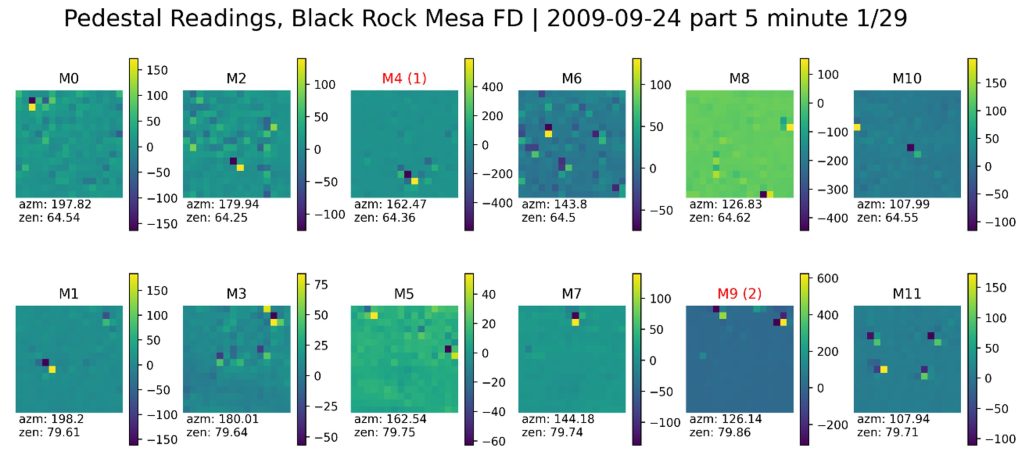
Figure 2.1 A signal change plot for the first minute of part 5 on September 24, 2009. Each of the twelve subplots represents a different mirror and displays a pixel for each PMT of the particular mirror. Red text indicates mirrors with chosen candidate stars in their field of view. The number in parentheses indicates the number of stars automatically selected within that mirror for further analysis.

Next, we sought to identify each chosen star by name. For each chosen star, we recorded the specific PMTs it passed through. Because the elevation and azimuth of each PMT in the detector are known, we were able to determine the elevation and azimuth of the star at a specific time. Then, using the geographical location and elevation of the observatory, we used the AstroPy module in Python to perform a coordinate transformation from Altitude-Azimuth or “Alt-Az” coordinates to celestial coordinates, which gave us the right ascension and declination of the star in question.

Once we calculated the celestial coordinates of a particular star of interest, we used a module called Astroquery to perform a cone-shaped search starting at these coordinates. This module searches in a cone around the specified celestial coordinates and returns astronomical objects within that cone, based on a specified catalog. In our case, we chose a cone with a radius of two degrees, and searched from the “HST Guide Star Catalog, Version GSC-ACT 1”. We found that this method resulted in a good balance between accuracy, reliability, and computer processing efficiency. Using a smaller radius resulted in an occasional failure to find the correct star, whereas using a larger radius resulted in exceedingly long search times.

From the list of astronomical objects returned, the target with the brightest magnitude was predicted to be the object responsible for the signal. This magnitude was recorded, as well as the “GSC ID” for the star, which is a ten-digit identifier based on the Guide Star Catalog, which we use as our database of possible celestial targets. From our experience, only stars of magnitude brighter than 2.50 or so result in high-quality decay fits. Therefore, we kept only stars with a magnitude brighter than 3.00 for further analysis. For each minute of each part of the data we analyzed, we recorded the PMT number of each star that fit these criteria. As each part of each night was automatically analyzed, we generated a list of PMTs through which each star passed. In order to be liberal with the selection of PMTs for further analysis, for each tube recorded in this list, we included all of the neighboring tubes in that same mirror.

At the end of this phase, we had generated a list of stars that we wished to analyze further, as well as a list of tubes through which each star passed on each particular night.

Then, in order to generate a decay fit for a particular star on a particular night, we plotted the signals of all these tubes together. To do this, we performed baseline subtractions to account for systematic differences in the baseline signal for different tubes [2]. The baseline was gathered from a 150- minute time interval average before and after the main pulse was detected in the tube. The signals in the first 30 minutes before and after the pulse were excluded, so as to not include the signal itself in the average. This resulted in a baseline calculated from a total of 240 minutes.

The time for the horizontal axis of the resulting plot is shown in UTC. Because the signals are in one-minute intervals, the UTC for each signal was calculated using the recorded start time for each part of data taken, and the time elapsed since the beginning of the part. When the signals for all tubes are plotted together, the resulting plot looks as follows:

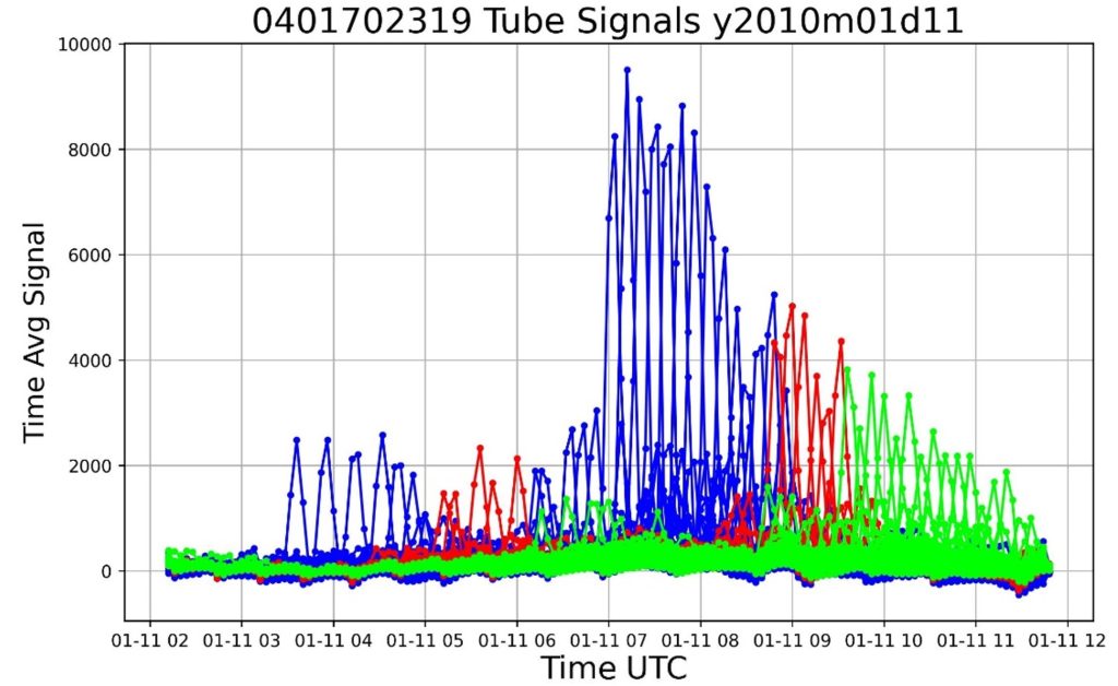Figure 2.2: Tube signal plot for a star with a GSC ID of 0401702319 (γ Cassiopeiae), observed on January 11, 2010. Each individual pulse represents the signal from one tube. Different colors correspond to different mirrors of the observatory. The time is in mm-dd hh format.

In this plot, each individual tube creates an individual pulse. Tubes of the same mirror are grouped together by color, showing when the signal passes through different mirrors as the star travels across the sky. As the star approaches the horizon over time, the peak value of each tube becomes smaller due to increased atmospheric light scattering. The upper edge of these individual pulses forms a decay function, which is what we wish to analyze. When determining how to analyze this behavior, we considered two possibilities: whether to perform minute-by-minute summations of the signals of the tubes or, alternatively, to fit only the peak pulses of individual tubes. We decided to try both methods and found that fits for the individual tubes resulted in more precise results and higher-quality fits. Therefore, this is the method we ultimately chose to adopt.

Once we obtained the data for fitting, we had to establish a physical model on which to base the fit. Atmospheric scattering can be described as a function of the optical depth 𝜏 by the following relation [4]:

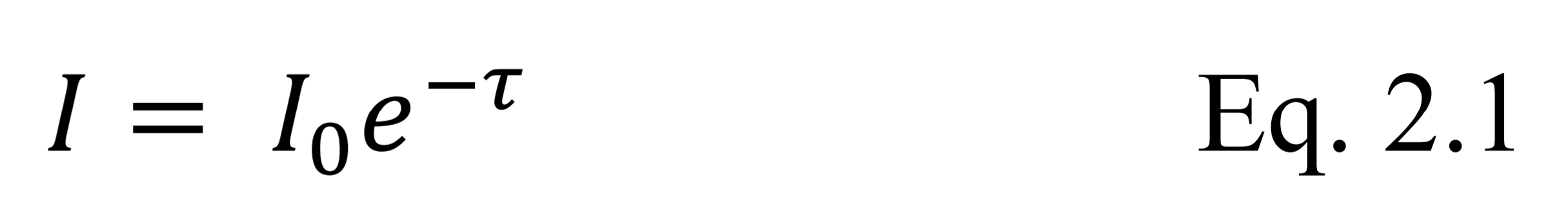
Where 𝐼 is the intensity of light that is observed after it undergoes scattering, and 𝐼₀ represents the intensity of the light before it interacts with the atmosphere. This relation is based upon a model where each particle scatters some proportion of light. If there are many particles between the incident light and the detector, as there are in the atmosphere, the measured intensity is an exponentially decaying function of the optical depth 𝜏. The optical depth is a measure of the number of particles that scatter the incoming light.

Even under constant atmospheric conditions, the optical depth varies as a function of the elevation angle. At lower elevation angles, starlight must pass through a relatively thicker atmosphere before it reaches the fluorescence detectors at the TA, which is equivalent to a larger optical depth.

This is the effect responsible for the red color of sunsets. As the Sun approaches the horizon, its light undergoes progressively more scattering. Because blue light is subjected to scattering to a larger extent than red light, the Sun gives off a red glow as it sets.

This also explains the starlight signal intensity decay we observe in the plot of tube signals over time. If we make a flat-Earth approximation, we can describe the optical depth as a trigonometric function of the elevation angle. 𝜏₀ represents the optical depth when measured vertically, which is known as the vertical optical depth or VOD. This approximation is shown in the Fig. 2.3 below:

Figure 2.3    Flat-Earth approximation of the atmosphere, with the vertical optical depth (VOD) shown as 𝜏₀, and an optical depth 𝜏₁ at elevation angle 𝜃.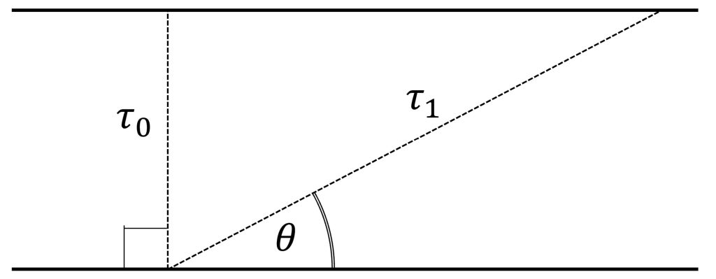

With some simple trigonometry, we arrive at the following relation between 𝜏₀, 𝜏₁, and 𝜃:

By rearranging the terms, and converting sin 𝜃 to csc 𝜃, we obtain:

If we substitute this relation into our intensity calculation in Eq. 2.1, treating 𝜏₁ as the optical depth 𝜏 at some elevation angle 𝜃, we obtain the following function:

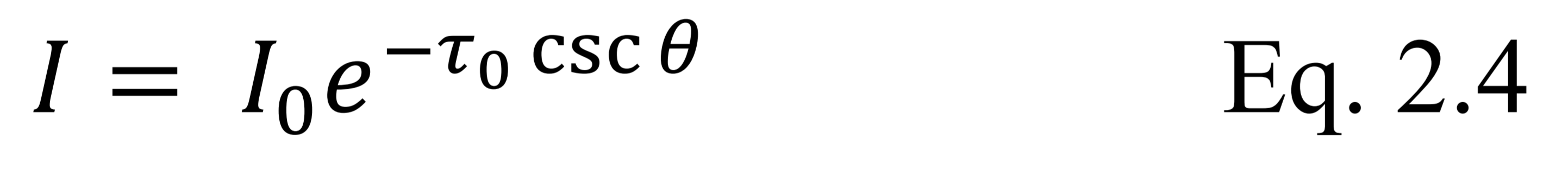
Where 𝜏₀ represents the vertical optical depth, 𝐼₀ represents the intensity of the starlight before it interacts with the atmosphere, and 𝜃 is the elevation angle of the star observation made by the fluorescence detector.

We predict that 𝜏₀, the VOD, should be a function of the current atmospheric conditions, and, ideally, should be equal between different stars under identical atmospheric conditions. Therefore, this parameter should vary primarily with time––more fundamentally the current atmospheric conditions, namely the aerosol concentrations––and be independent of the star used to calculate it. Because 𝜏₀ represents a direct estimate of the atmospheric transparency and is independent of the intrinsic magnitude of the star used to calculate it, it is the parameter we are most interested in.

The next step was to perform fits between Eq. 2.4 and the data obtained from various stars on various nights. The tube signal data in Fig. 2.2 is plotted with signal strength–which is proportional to the measured intensity–on the vertical axis, and time on the horizontal axis. However, Eq. 2.4 expresses the intensity as a function of the elevation angle, not time. Thus, we needed to transform the horizontal axis to show the elevation angle–instead of the time–at which the signals were recorded.

Because the elevation and azimuth angles of each PMT in the detector are known, we developed a script that assigned an elevation angle to each signal, based on the tube number and mirror number that the signal was recorded in. Once this was accomplished, we were able to plot the measured signal strength as a function of the elevation angle for each individual star on a given night being analyzed. An example plot is shown below:

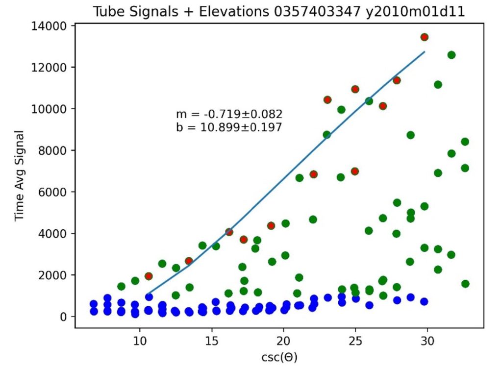
Figure 2.4 Plot of selected signals and the fitted model for a star with a GSC ID of 0357403347 (Deneb). Signals below 1000 are excluded from the fit and are shown in blue. Local maxima of all remaining signals are used for the fit and are highlighted with red.

For each night, a list of tubes was made through which the given star passed. Because signals from each tube were recorded both before and after the starlight passed through them, these signals also appear in Fig. 2.4 as baseline signals. In order to eliminate these from the fit, signals below 1000 were excluded and are shown in blue. The remaining signals are shown in green. There are also many intermediate signals in each tube, before and after the peak of the pulse. Because we are only interested in the peak of each signal pulse, we devised a method to filter out as many of these intermediate signals as possible.

To do this, we grouped the green data points in groups of five and only included the local maximum value of each group in the fit. These chosen values are indicated with a red point in the fit and are the only points used in fitting the model to the signal data.

Fig. 2.4 also shows the fitted model with a blue line, which was generated by a script that linearized the data and applied an optimized linear fit using the scipy.optimize.curve_fit function from the SciPy module. Because Eq. 2.4–the equation we use to model signal intensity decay–contains an exponential, as well as a csc 𝜃 term, we elected to linearize the data in order to make the fitting vastly more efficient. To accomplish this, we transformed the signal intensity to a logarithmic scale and plotted the horizontal axis as the cosecant of the elevation angle. In this way, the model in Eq. 2.4 became linear, which greatly streamlined the SciPy curve fitting process. The error bars were determined based on the amplitude of the fluctuation in the signal baseline. These error bars, along with the fit quality, were used by the curve fitting function to calculate the uncertainty in the optimized fit parameters. A plot of this linearized data for one star on one night, along with the optimized linear fit, is shown:

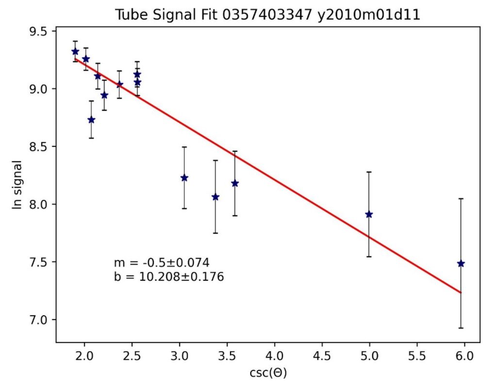
Figure 2.5 Linearized data and the linear fit for the star Deneb, with the slope m and intercept b calculation. The absolute value of the slope corresponds to the 𝜏₀ parameter, or VOD. The intercept of the fit corresponds to the 𝐼₀ parameter.

For reference, the equation with which we model the signal intensity decay is as follows:

In the linear fit, we obtain two parameters: the slope m and the intercept b, along with the uncertainties for each. These parameters correspond to −𝜏₀ and 𝐼₀, respectively. Flipping the sign of the slope m gives the VOD, and the intercept b corresponds to 𝐼₀, which is the estimated intensity of the starlight before interacting with the atmosphere.

By repeating this process for several nights, we generated a list of VOD parameters, each corresponding to a given star on a given night. We examine the results in the following section.

Results

In total, we analyzed data from 26 nights, and thereby generated data for over 70 stars. Of these stars, approximately half had five or more successfully generated VOD parameters. These parameters were only calculated when the star had three or more data points from which to generate a fit. In total, we obtained 306 VODs, with uncertainties calculated for each by the scipy.optimize.curve_fit function based on the quality of the fit, and the error bars.

We elected to create a histogram of this data to visualize the distribution. We exclude VODs with uncertainties greater than 100%; this implies a low confidence fit. Furthermore, we exclude VODs that are greater than two, and less than zero.

A VOD of less than zero implies that the signal intensified as the starlight was scattered by more of the atmosphere, which is certainly incorrect. A case-by-case analysis of the particular fits that generated negative optical depths revealed that these fits were based on highly incomplete and noisy data, which confirms our reasoning that these cases do not accurately represent meaningful physics, and are therefore rejected.

A VOD of greater than two implies a very quick extinction of the signal, too quick to be a reliable VOD based on atmospheric light scattering alone. Calculated VODs with values of greater than two are likely to be caused by a cloud obscuring the star from view or simply by the star leaving the field of view of the detector. Therefore, we choose to reject these values as well.

After excluding VODs based on the above criteria, we generated the following histogram:

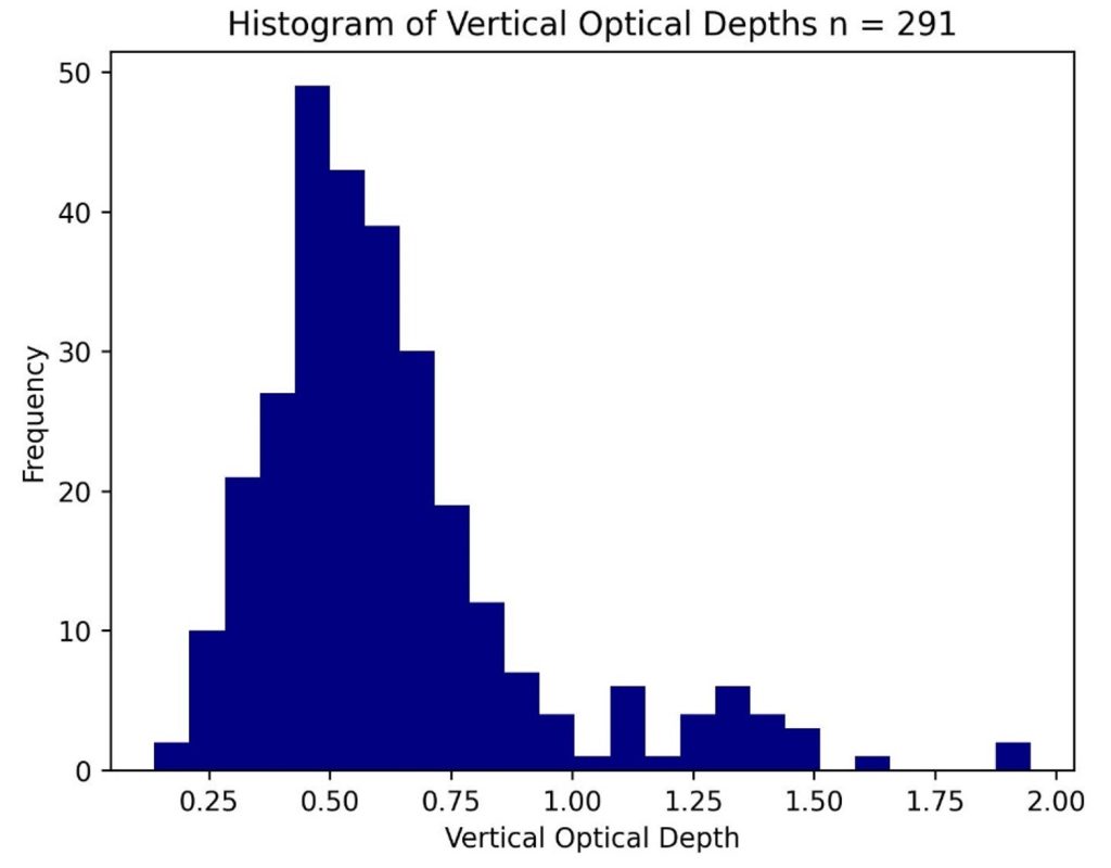Figure 3.1 Histogram of calculated vertical optical depths, with 291 total values. The mean is 0.623, and the standard deviation is 0.290.

In total, the histogram in Fig. 3.1 represents the calculated VOD from 48 stars, taken over 26 nights. The smallest recorded VOD was 0.137. We can use Eq. 2.4 to deduce what this value implies:

Because 𝜃 is the elevation angle, a vertical measurement means that 𝜃 is equal to 90 degrees, which implies that csc 𝜃 becomes equal to unity. In this case, the equation reduces to the following:

If we substitute the calculated VOD for 𝜏₀ and rearrange, we obtain the following relation:

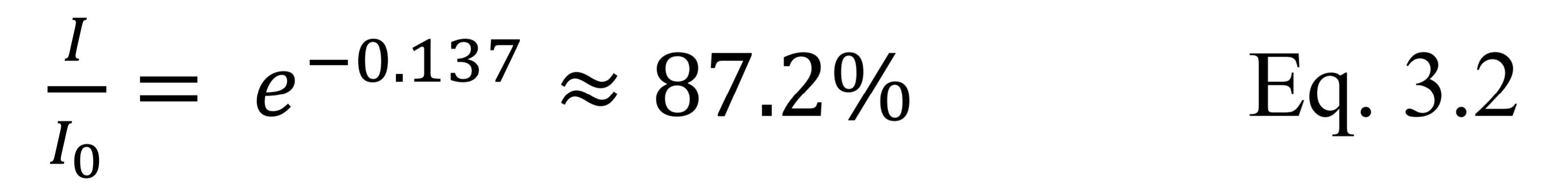
This means that during the period in which the particular star was observed, the atmosphere was estimated to have an 87.2% vertical transmission factor of light in the 300 to 420 nm band.

The mean VOD is 0.623, and the standard deviation of the set of VODs is 0.290. By Eq. 3.2, as above, a VOD of 0.623 implies a mean vertical atmospheric transparency of approximately 53.6% in the 300 to 420 nm band.

In order to assess whether or not these calculated VODs are reliable indicators of a meaningful physical property, we analyzed the calculated VODs in conjunction with the night on which they were measured, looking for night-to-night correlations within the data. We expected the calculated VODs to be conserved between the decay fitting of different stars at the same time. To maximize the statistical reliability of our analysis, we focused on stars with five or more calculated VODs. In other words, these are stars that were successfully observed on five or more nights with highly reliable fits. In total, this set consisted of 24 individual stars. From this set, we noticed that there were two stars with VOD parameters that appeared very closely correlated from night to night: Alioth and Alkaid, which are the first and third brightest stars in the Ursa Major constellation, respectively, forming part of the “handle” of the Big Dipper.

In order to test this observation, we generated a plot of the calculated VODs versus the night on which each particular VOD was measured. The horizontal axis is not necessarily spaced evenly in time; because certain stars appear in the field of view of the detector only at particular times of the year, the intervals between some measurements are on the order of a day or two, while others may be close to a year apart. In total, we found eleven nights on which high-confidence VODs were calculated for both Alioth and Alkaid:

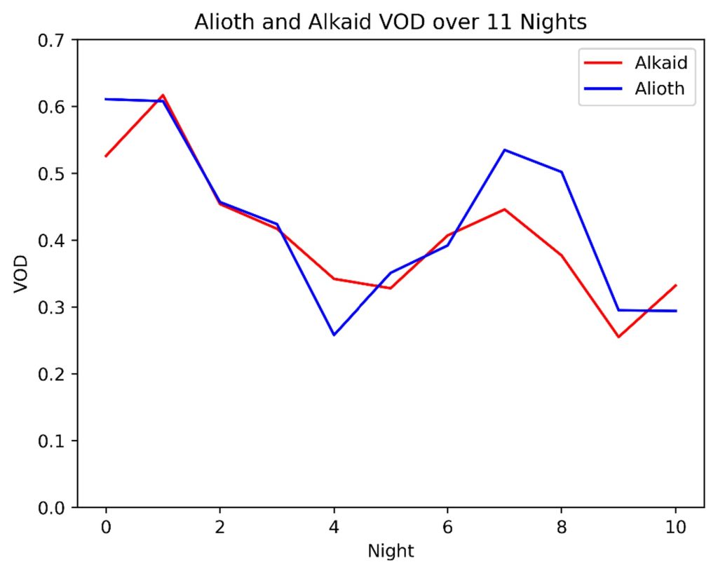Figure 3.2  Calculated VODs for Alioth and Alkaid, with data from 11 individual nights.

It is clear that the trend in the VOD is very similar between the two stars. This correlation suggests, at the very least, the existence of a common time-dependent factor that influences the signal intensity decay of these two independent stars. In order to quantify this relationship, we generated a correlation plot, with the VOD of Alioth on one axis, and the VOD of Alkaid on the other axis. The result is shown below:

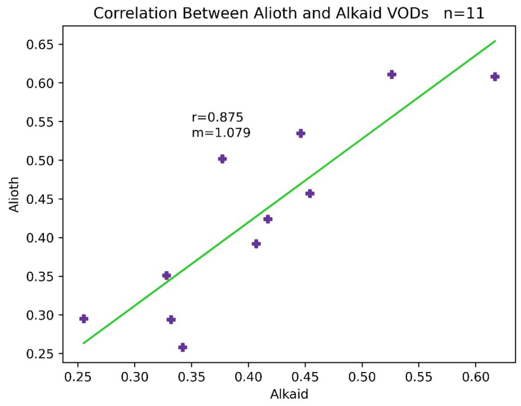Figure 3.3 Calculated VODs for Alkaid on the horizontal axis, and VODs for Alioth on the vertical axis, with 11 total data points. The correlation coefficient r and slope of the linear fit m are shown.

The calculated correlation coefficient for the linear regression is 0.875. Using this correlation coefficient along with the number of data points, we can evaluate the statistical significance of this observed correlation between these two stars. This case has 11 data points–and therefore 9 degrees of freedom–which, if we adopt a 99% confidence level, implies that the critical value for the correlation coefficient is 0.735 [5]. Because the calculated correlation coefficient of 0.875 is significantly above this critical value, we claim with 99% confidence that a statistically significant correlation exists between the calculated VODs of Alioth and Alkaid on these 11 nights.

Discussion

Now that we have demonstrated a statistically significant relationship between the VODs calculated from the signal decay of two independent stars, we can confidently claim that there is a common time-dependent factor that influences these decay functions uniformly. However, two important questions remain.

First, what is this common factor, and what additional work can be done to definitively link a specific variable to starlight signal decay–and more fundamentally–the transparency of the atmosphere?

Our project shows that starlight signal decay, caused by atmospheric light scattering, can be used to estimate the VOD of the atmosphere. This atmospheric light scattering has been shown by our methodology to change in time, as shown by the correlation in VODs of two different stars, calculated on the same nights. Because light scattering is caused primarily by Rayleigh scattering and aerosol scattering, we can predict that one of these phenomena is responsible for the observed variation in VOD. Because the VOD has been shown to change in time–and the Rayleigh scattering component is approximately constant in time–we primarily attribute the observed VOD changes to aerosol scattering, which is variable.

However, more work is required to show a definitive link between atmospheric aerosols and the VODs calculated by this starlight decay fitting technique. Specifically, what is needed is a set of data from the approximate location of the Black Rock Mesa site of the TA that contains the concentrations of various aerosols, as well as their respective particle sizes, in order to estimate the expected scattering in the 300 to 420 nm range. Then, if this data is overlayed against the VOD calculations obtained by our method, a specific relation can be established between the measured aerosol concentrations at a given time and the expected effect on the measurements taken by the TA observatory.

There is also a second question that is raised by our results. Of the 24 stars that we analyzed for VOD correlations, only 2 showed high-confidence correlations between the VOD values calculated on the same nights; what are possible explanations for this?

Our project originally began with the expectation that the VOD stays relatively constant during a certain night, with significant differences observed between separate nights. This would imply that the VOD calculated from all stars on a given night should be correlated. However, we believe that our results suggest otherwise. The two stars that we found to produce well-correlated VOD values are part of the same constellation, Ursa Major, and appear quite close together in the night sky. Therefore, their signal intensity decay is recorded by the TA during an almost identical time interval. On the other hand, other stars enter and exit the field of view of the detector at different times throughout the night. One possible explanation for the lack of convincing correlations between other stars is that the atmospheric aerosol concentrations vary significantly not only from night to night but also during the course of a certain night. Therefore, stars that are observed during similar time intervals may show similar decay behavior and therefore result in similar VOD calculations, whereas stars that are further apart are likely viewed during different atmospheric conditions. Therefore, while we believe that our starlight decay fitting method does in fact produce convincing estimates of the current VOD, and conversely the atmospheric aerosol concentrations at a given time, we do not believe that the VOD calculated by the observation of a single star can be used to estimate the VOD of the entire night. Instead, we believe that the calculated VOD is only reliable during the interval in which the star was observed, which is typically on the scale of a few hours. For this reason, we believe a promising prospect for future work includes the measurement of atmospheric aerosols in finely spaced time intervals, on the order of an hour or finer, and subsequent comparison with the calculated VODs obtained by analyzing starlight signal decay.

However, even at this present stage, we are confident that we have shown convincing evidence that atmospheric changes do in fact produce measurable and significant changes in the light detected by the fluorescence detectors at the Black Rock Mesa site of the TA. Therefore, we believe that atmospheric effects should be taken into account during data collection at the TA in general, in order to allow for more accurate detection of cosmic rays and other cutting-edge phenomena in physics.

References

[1] D. Furlich, Observation of the GZK Suppression with the Telescope Array Fluorescence Telescopes and Deployment of the Telescope Array Expansion, PhD Thesis. (University of Utah, Salt Lake City, 2020).

[2] Siddique, University of Utah REU 2020 Summer Research Program Project Summary. (University of Utah, Salt Lake City, 2020).

[3] J. Cox, A. J. Deweerd, and J. Linden, An experiment to measure Mie and Rayleigh total scattering cross sections. Am. J. Phys. 70(6), 620 (2002).

[4] W. Lui, M. Clarkson, R.W. Nicholls, An approximation for spectral extinction of atmospheric aerosols. Journal of Quantitative Spectroscopy and Radiative Transfer. 55(4), 519 (1996).

[5] Niño-Zarazúa, Quantitative Analysis in Social Sciences: An Brief Introduction for Non- Economists. SSRN Electronic Journal (2012).