8 Chapter 8: Learning from Oxymorons II – Industrial Ecology
If finance represents the circulatory system of an economy, industrial ecology is the digestive tract. It’s about industrial throughput and metabolism, what happens at the back door of restaurants and stores, on farms and in food-processing plants, in factories, power plants, and mines. You may have been introduced to industrial ecology through the idea of footprint such as ecological or carbon footprint. As a positive science, industrial ecology analyzes and quantifies the flow of natural resources and energy through the economy to produce specific goods and services. If you’re like others, you’ll be amazed by the volume of natural resources you consume, most of it indirectly in the bowels of industrial and agricultural production and supply chains. As a normative strategy, it identifies how the economy’s digestive tract can go on a diet, reducing the use of natural resources and energy used, and the waste produced, to achieve important results. Taken to an extreme, we can even talk of dematerialization, where little energy and few material goods are needed to perform many services. For example, as we have seen in response to the Covid-19 pandemic, communication can often substitute for transportation and need not consume paper, though it usually requires some electricity.
We’ll start this chapter by taking a look at an energy and material flow analysis of the U.S. as compared to the European economy. After all, the Mecca of industrial ecology is the Institute for Social Ecology in Vienna, Austria. The Germanic-speaking countries of north-central Europe are leading the way among industrial regions in using natural resources most efficiently by employing industrial ecology principles. We’ll then look more closely at the popularized versions of footprint analysis—ecological footprint, carbon footprint and water footprint—identifying their strengths and weaknesses. Next we’ll apply these concepts in an in-depth industrial ecology analysis of a controversial product—corn-based ethanol. We’ll finish with a discussion of how energy and material use can be reduced, making economies leaner and meaner from a natural resources point of view.
Energy and Material Flow Analysis
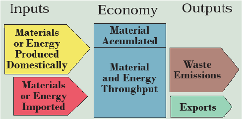
What do we mean by energy and material flow through an economy? Figure 8.1 shows this in simple form where domestically produced and imported raw materials and energy feed into the economy and waste emissions and exports flow out of it. Most of the material is throughput, but some materials may accumulate in manufactured capital, like wood in buildings or aluminum in airplanes. Most of the work in doing flow analysis lies in measuring and quantifying, and in so doing, methodological rules have to be developed. For example, is soil eroded during crop production counted as throughput? How about rain falling on the grass pastures cattle graze? Different analyses may yield different results because of variations in how these kinds of rules are applied. The devil can therefore lie in the details and we need to look at more than just the bottom line but at what the flows actually represent.
You may have heard that Americans consume more than their share of natural resources. What does an energy and material flow analysis show? Table 8.1 compares the U.S. economy to that of the 15 member nations of the European Union as of 2000 (EU-15), a region of the world that enjoys a similar standard of living as the U.S. with a slightly larger population (361 million in 2000 compared to 281 million in the U.S. in that year).
We’ll start with energy, including the energy content of food and wood from biomass as well as electricity and fossil fuels. In 2000 the U.S. consumed 125 exajoules (see Table 8.2 on energy units) compared to 79 in the EU-15 but more than twice as much per person (445 gigajoules vs. 210 GJ). The U.S. also imported slightly more per person (118 GJ vs. 102 GJ) even though the U.S. met a smaller total proportion (20 percent) of its energy needs from imports than did the EU-15 (40 percent). The mix of sources was similar, with the greatest reliance being placed on fossil fuels, but the EU-15 relied about twice as much on nuclear energy than the U.S., largely due to France’s extensive nuclear power program.
Table 8.1. Comparison of U.S. and European Union energy and materials flows in 2000.
Sources: Weisz et al., 2006; Haberl et al., 2006.
|
|
U.S. |
EU-15 |
|
Energy Flow Analysis |
||
|---|---|---|
|
Domestic Energy Consumption (EJ/yr) |
125 |
79 |
|
Domestic Energy Consumption (GJ/capita/year) |
445 |
210 |
|
Imports (GJ/capita/year) |
118 |
102 |
|
Percentage from: |
||
|
Biomass (including food) |
20 |
23 |
|
Fossil Fuels |
73 |
63 |
|
Nuclear |
6 |
13 |
|
Renewables |
1 |
1 |
|
Imports |
20 |
40 |
|
Biomass Energy Consumption (GJ/cap/yr) |
88 |
50 |
|
Percentage of Net Primary Production Harvested |
>15 |
>28 |
|
Energy Consumed per dollar GDP (1980) (MJ) |
24 |
17 |
|
Energy Consumed per dollar GDP (2000) (MJ) |
16 |
12 |
|
Material Flow Analysis (tonnes/capita/year) (percent imported) |
||
|
Biomass |
7.0(-) |
4.0 (5) |
|
Construction materials |
No data |
7.0 (0) |
|
Industrial minerals and ores |
No data |
1.0 (60) |
|
Fossil fuels |
12.2 (20) |
3.7 (49) |
|
Total |
>19.2 (-) |
15.7 (17) |
Table 8.2. Understanding units of measure for energy.
|
Metric Unit: Joule: the energy to raise the temperature of 2 kg of water from 0oC to 1oC. |
||
|
English Unit: British Thermal Unit (BTU) = 1,054 joules |
||
|
Prefix |
Exponent |
English word |
|
nano |
10-9 |
billionth |
|
micro |
10-6 |
millionth |
|
milli |
10-3 |
thousandth |
|
centi |
10-2 |
hundredth |
|
deci |
10-1 |
tenth |
|
deka |
10 |
ten |
|
hecto |
102 |
hundred |
|
kilo |
103 |
thousand |
|
mega |
106 |
million |
|
giga |
109 |
billion |
|
tera |
1012 |
trillion |
|
exa |
1015 |
quadrillion |
The biomass component of energy consumption is interesting because it reflects important geographic and ecological relationships that we will explore below under Ecological Footprint 2.0. Europe is more ecologically productive per unit area because of the vast dry areas in the U.S. West and cold areas in Alaska. It’s four times more densely populated, however, leaving less biological productivity per person. Europe’s 50 GJ of biomass energy consumption per capita is similar to other regions around the world, developed and developing, and reflects ecological requirements for food, fiber, and other basic needs. The per capita figure for the U.S. is higher (88 GJ) because Americans have inherited a great store of natural capital that they use liberally by eating meat-rich diets, building big wooden houses, and so forth. Europeans consume or appropriate at least 28 percent of the net primary production of their territory in this manner and are net importers of biomass while Americans appropriate at least 15 percent and are net exporters. Here we can see the extra “elbow room” that Americans enjoy in the sense that the human population is not pressing as hard against the ecological carrying capacity of the land as it is in Europe.
Each year, the average European consumes 4 metric tonnes of biomass (mostly in the form of agricultural and wood products), 7 tonnes of construction materials (e.g., concrete, sand and gravel, brick, paint), 1 tonne of industrial minerals and metallic ores, and 3.7 tonnes of fossil fuels (oil, gas, and coal). For materials, U.S. data comparable to those from the EU-15 are lacking, but fossil fuel and biomass comparisons can be generated from the energy data. They show 7 tonnes of biomass and 12.2 tonnes of fossil fuels. If the U.S.-EU ratios on construction materials and ores are similar, the average American consumes roughly 40 tonnes of materials per year, about 600 times their body weight. Over their lifetime, an American will consume over 3,000 tonnes, 45,000 times their body weight. And this does not include air and water. Only 6 percent of natural resources extracted end up in products, and only 1 percent in durable products. The rest is throughput. Only a few percent of the energy content of fossil fuels at the power plant provides light, washes dishes, or cools food. Less than 1 percent of the energy content of gasoline moves the driver forward (see derivation in Chapter 14).
Why is the European economy more energy- and resource-efficient than the U.S. economy? A large part of the answer is that the U.S. economy has evolved under conditions of greater natural resource abundance than Europe’s. In fact, since 1980 both economies have begun to use fewer resources per dollar of gross product produced or, to put it another way, total energy and resource consumption have remained fairly constant despite population and economic growth. Using energy as a measure, the U.S. used 24 MJ of energy per dollar of gross product in 1980 but only 16 MJ in 2000 while the European economy improved from 15 MJ in 1980 to 12 MJ in 2000. So as the historic natural resource abundance of the U.S. has diminished, it has been catching up to Europe in resource use efficiency. This is the powerful ecological modernization trend that industrial ecology can help to continue and even accelerate. It is by reducing the need for raw materials and energy to maintain our welfare that natural resources sustainability can be achieved.
Footprint Analysis: Ecological, Car-bon, Water
Footprint analysis traces back the natural resources needed and the pollutants emitted in the production of specific products or for entire regional or national economies. It has become the popular face of industrial ecology and can teach us about how our lifestyles impact the planet. We also need to ask a lot of questions, however, about what the numbers really mean. Let’s explore ecological, carbon, and water footprints.
Ecological Footprint 1.0
Mathis Wackernagel and William Rees developed the ecological footprint concept in the 1990s as the area of ecologically productive land and ocean that is required to continuously provide the resources consumed by a group of people (such as a country) and to process their wastes. According to their analysis in 1999, the average person in the world uses about 6 to 7 acres. Indians use only 2 acres, Chinese use only 3, Germans 13, Canadians 19, and Americans 25, the highest among any nation in the world. Moreover, the world only contains 5 productive acres per person, implying that we are overshooting our collective carrying capacity. Americans are using 9 of their 25 acres either from beyond their borders (by importing natural resources and exporting wastes) or by borrowing natural capital from the future. Canada, in contrast, has an ecological surplus.
We can also analyze the composition of the ecological footprint of the average person and how this is changing over time. Each of us utilizes the renewable resource capacity of land through our diet (crops, pasture, and fisheries), raw materials (forests), land developed for our use (urban land), energy needs (fuelwood and carbon dioxide absorption), and land contaminated by nuclear weapons and power development. Over time, the average footprint expanded from 1960 to 1980, but it has remained about stable since then as declining land requirements for crops has balanced increasing land needed to sequester the carbon dioxide emitted when we use energy.
These are interesting comparisons, and they illustrate important trends, but they are not without conceptual weaknesses. Why use an acre of generic land as a unit of analysis when ecosystems vary so enormously from place to place as we saw in Chapter 4? For food production the relationship is somewhat straightforward, but can we convert, for example, coal mined from the Earth, burned in a power plant, and emitting carbon dioxide into the atmosphere into an equivalent land area? Would this be the area of land required to absorb the carbon dioxide through photosynthesis? But what if the carbon dioxide is sequestered in geologic formations or simply left in the atmosphere as a greenhouse gas? Is nuclear area determined by the area left unfit for habitation by the Chernobyl accident and other nuclear wastes derived from weapons programs in the U.S. and the old Soviet Union?
There is also a problem of geographical specificity. Which land and ocean areas are supporting which people? Could you place your 25 or some other number of acres on a map? Moreover, generally only provisioning ecosystem services and waste processing “consume” land, and then only partially and temporarily while cultural, regulatory, and supporting services can be provided for large groups of people simultaneously and continuously from a single ecosystem. I’m left with regarding ecological footprint as a useful but seriously flawed tool of industrial ecology because it is divorced from the actual cycles (e.g., carbon, water, nitrogen, energy) that are affected by resource use and from the economic values, positive or negative, of human impacts on those cycles. Fortunately, we have a better approach: human appropriation of net primary production.
Ecological Footprint 2.0: Human Appropriation of Net Primary Production
One mark of a scientifically sound and valuable footprint measure is that it is directly linked to Earth’s key biogeochemical cycles and ecological processes that we studied in Chapter 3 and 4. Net primary production emerges as the key measure of an ecosystem’s capacity to photosynthesize and store biomass that, as the first trophic level, forms the foundation of the ecosystem. A measure of ecological footprint, then should focus on how humans utilize and impact this foundation.
In the 1980s, Peter Vitousek and colleagues calculated human appropriation of the products of photosynthesis. Conceptually identical but a bit more precise from the point of view of ecological energetics, human appropriation of net primary production (HANPP for short) has emerged in the 21st century as the most scientifically rigorous way to measure how humans, as the dominant species on the planet, are capturing their niche in the biosphere.
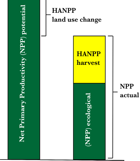
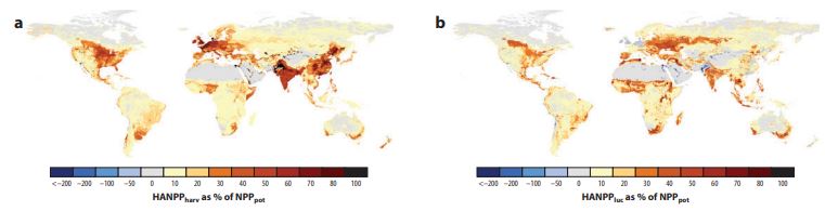
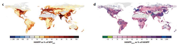
Figure 8.2 defines HANPP. We start with the rate of net primary production that an ecosystem could potentially achieve if humans were not affecting it. Because it’s a theoretical potential rather than a measured actual quantity, it has to be modeled or estimated based on climate, soils, topography, and other measures. When the actual NPP is measured from satellites like MODIS or Landsat, the difference between the two becomes HANPP due to land use change. Map (b) in Figure 8.3 shows HANPP(land use change) as a percentage of NPP(potential). This measures the degree to which human uses of land have diminished (through deforestation, overgrazing, fire, soil erosion, urbanization and so forth) and occasionally augmented (usually through irrigation), the capacity of the ecosystem. HANPP(land use change) is rarely a good thing and, in fact, we can use it to measure how ineffectively humans are using the land. Desertification is perhaps the epitome of HANPP(land use change) where centuries of overgrazing or poorly managed irrigation have rendered the ecosystem a shadow of what it once was. Remember the stripping of soil in the Mediterranean and Middle Eastern lands from Chapter 2 as well as America’s Dust Bowl.
From actual NPP, humans harvest the biosphere, primarily through cultivating crops, grazing livestock, and cutting timber from forests. All 7.8 billion humans on Earth are and always have been utterly dependent on HANPP(harvest) for all of their food as well as most of their needs for fiber (cotton, flax, hemp, wool, wood) and the biomass portion of their energy needs (wood, ethanol, etc). Map (a) in Figure 8.3 thus primarily reflects agricultural intensity. Map (c) shows total HANPP calculated as HANPP(land use change) plus HANPP(harvest). Densely populated and/or intensively farmed areas like India, eastern China, central Europe, and the American Midwest stand out as the ecosystems humans have appropriated to the highest degree. Map (d) shows the efficiency through which those impacts produce food, fiber, and biofuel that humans actually use.
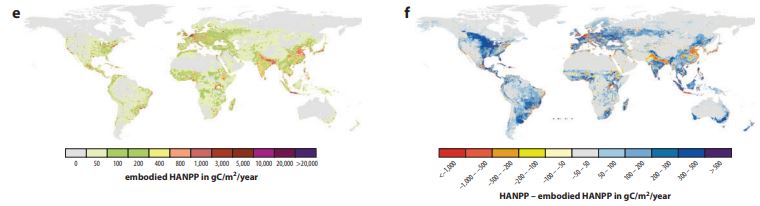
There was a day long ago when the ecological products—provisioning ecosystem services that humans rely upon for their survival—originated where they live or close nearby. Trade, increasingly globalized but also important within regions, has changed all that, and so in the 21st century, humans often rely upon distant ecosystems for their food, fiber, and biofuel. Map (e) shows the consumption of HANPP, called embodied HANPP. While hard to see at a global scale, most consumption of food, fiber and biofuel occurs in cities, where a majority of people now live. So, while in past centuries, the production of HANPP(harvest) and it’s consumption (embodied HANPP) would closely align, these are increasingly separated, with trade teleconnections along supply chains linking them together.
Finally, Map (f) shows the difference between HANPP production and consumption, so areas shown in blue are net HANPP exporters, while those in red are net importers. Of course, much of the map looks blue, because geographically large rural areas generally export HANPP, with the North American Midwest leading the way for the entire planet just as the Persian Gulf leads the way in oil exports. In the 21st century, eastern Brazil and northern Argentina has become the world’s second most important food and HANPP-exporting region. Meanwhile, every city on Earth is reliant on rural areas somewhere—regional hinterlands remain critical but increasingly from across the continent or even the planet—to supply its food, fiber and biofuel. In addition to cities, some large densely-populated regions are also dependent on imports, such as northern India, eastern China, Japan, the heart of Western Europe, the Middle East, and America’s eastern seaboard metropolis.
HANPP thus serves as a very perceptive lens through which we can explore ideas about ecological footprint with an expanded capacity to answer the critical questions: How much? How efficiently? From where? To where? How much nature is left? Compared to what it would otherwise be?
Carbon Footprint
Carbon footprint is straightforward because it takes one pool of carbon as bad—the atmospheric pool that drives climate change. Our carbon footprint is therefore the volume of carbon dioxide that our use of natural resources causes to accumulate in the atmosphere. While less severe than for ecological footprint 1.0, methodological issues remain. For example, why not also include the volume of methane released to the atmosphere (remember CH4 traps many times as much heat as an equivalent volume of CO2)? For this reason, CO2-equivalent is sometimes used. What parts of the life cycle of products do we include? For example, the gasoline burned in our car certainly counts, but what about the fossil fuels used to make the car, or that the workers who built it consumed driving to work?
If you type “carbon footprint” in Google you’ll get a long list of carbon calculators. One I find easy to use is Carbon Footprint Calculator. Table 8.3 shows how I calculated my carbon footprint at that website. At about 11.8 tonnes per year, my carbon footprint is just over half the U.S. average of 21.5 tonnes but more than twice the world average of 4.9 tonnes. My lower than U.S. average footprint is largely due to (1) I have solar panels installed on my roof, (2) I share a plug-in hybrid Prius with my wife and have a short 2-mile commute to work, (3) I don’t eat red meat unless it would be rude to refuse it, (4) I’m stingy about turning on the air conditioning in favor of ceiling fans, (5) I buy Energy Star appliances, and (6) I’m a pragmatic rather than a recreational shopper. On the downside, however, I really need to look at how I can use less natural gas to heat my home. Time to add insulation and caulk the windows! Then I can get to less than half the U.S. average and less than twice the world average (while saving on my monthly gas bill, especially in the winter). I’m sure you’re dying to calculate your own carbon footprint at this or another website, but also try some hypothetical scenarios to lower your footprint and see how large an effect they have.
Table 8.3. The author’s carbon footprint.
|
Component |
Relevant Data |
Footprint (metric tonnes per year) |
|---|---|---|
|
House |
2 people $700 on electricity $1,600 on natural gas |
2.02 4.16 |
|
Flights |
3 round trips of about 1,000 miles each way |
0.84 |
|
Toyota Prius |
Plug-in hybrid 12,000 miles driven |
1.41 |
|
Honda CR-V |
6,000 miles |
1.67 |
|
Food |
white meat and fish, some organic, prefer local produce |
1.66 |
|
Goods |
I buy new clothes, furniture, and electronics only when needed but avoid fancy packaging, drive to recreation sites, and use standard financial services, recycle, or compost about half of household waste |
|
|
Total |
11.76 |
Table 8.4. The U.S. carbon footprint in 2017.
| Sector Item | GHG Emissions (million tonnes) | % | GHG Emissions (million tonnes) | % |
| Transportation | 1,866 | 28.9 | ||
| Light-duty vehicles | 1,111 | 17.3 | ||
| Medium- and heavy-duty vehicles | 426 | 6.6 | ||
| Aircraft | 167 | 2.6 | ||
| Rail | 37 | 0.6 | ||
| Boats and ships | 37 | 0.6 | ||
| Other transport | 74 | 1.2 | ||
| Electricity | 1,778 | 27.5 | ||
| Industry | 1,435 | 22.4 | ||
| Fossil fuel combustion | 771 | 12.0 | ||
| Natural gas and oil systems | 260 | 4.1 | ||
| Other industry | 405 | 6.3 | ||
| Agriculture | 582 | 9.1 | ||
| Crop cultivation | 287 | 4.5 | ||
| Livestock | 256 | 4.0 | ||
| Fuel combustion | 40 | 0.6 | ||
| Commercial | 416 | 6.5 | ||
| Fossil fuel combustion | 235 | 3.7 | ||
| Landfills/waste services | 131 | 2.0 | ||
| Fluorinated gases | 51 | 0.8 | ||
| Residential | 331 | 5.2 | ||
| Fossil fuel combustion | 301 | 4.7 | ||
| Fluorinated gases | 40 | 0.6 | ||
| Land Use and Forestry | -714 | -11.1 | ||
| Total | 5,694 | 88.9 | 6,408 | 100.0 |
Leaping scales from the individual to the nation, the U.S. carbon footprint of about 6.4 billion tonnes annually is summarized in Table 8.4, where electricity from fossil fuel combustion and transportation contribute about 28 percent each, followed by industry, agriculture, and commercial and residential emissions. Land use and forestry, largely the ongoing growth of trees in the eastern U.S., offsets 11 percent of emissions.
The greatest reductions in the U.S. carbon footprint can be found in:
- replacing coal as a source of electricity with lower-carbon (e.g., natural gas) and no-carbon (e.g., nuclear, wind, solar) alternatives;
- reducing fuel use in vehicles, such as by improving gas mileage or replacing car and plane traffic with hybrids and trains;
- reducing fossil fuel use in industry;
- reducing methane emissions from landfills and agriculture;
- making land use and forestry an even larger carbon sink.
We’ll see this issue again when discussing our steep challenges in energy.
Water Footprint
It is perhaps understandable to exclude air and oxygen from energy and material flow analyses because they are so ubiquitous, but fresh water is a critical input to agricultural and industrial production and is not nearly so abundant. Many products contain water embedded within them, but more meaningful is the amount of water that is used to make a product. The amount of water we drink (perhaps one gallon per day) or even use from the faucets, showerheads, toilets, and other household appliances where we live (an average of 70 gallons per day in the U.S.) is trivial compared to the amount of water that is consumed to produce our food and energy. In the U.S., irrigation accounts for 40 percent of water withdrawals and 83 percent of water consumed. Thermoelectric power generation—cooling coal, nuclear and natural gas power plants to keep them from melting when they generate electricity—accounts for 39 percent of withdrawals but only 1 percent of consumption because the water usually goes back to its source—albeit quite a bit warmer. Moreover, if we count rainfed agriculture, 94 percent of our water footprint comes from the food and other agricultural products we consume because of the high rates of transpiration in crops and the large areas that are planted to them.
Given these data, food products have the highest water footprint, especially meat products reflecting the conversion ratios of feed to animal weight. Products like coffee and cotton, where only a small proportion of the crop is used in the final product, also have high footprints. Table 8.5 clearly shows how to reduce your water footprint—simply start at the top and work your way down. (I say this to you while drinking coffee and wearing a cotton shirt and pants!) Yes, you should turn off the faucet while brushing your teeth, but if you really want to make a difference by conserving water, look at Table 8.5 and have a tomato or two for lunch instead of a hamburger and orange juice.
Table 8.5. Water footprint as mass ratios (weight water: weight product) for common agricultural products in the U.S. Source: Chapagain and Hoekstra, 2004.
|
Product |
Water Footprint (mass ratio) |
Product |
Water content (gallons) |
|
Beef |
13,193 |
Pair of leather shoes |
2,100 |
|
Coffee |
5,790 |
Cotton T-shirt |
1,100 |
|
Cotton |
5,733 |
Hamburger |
630 |
|
Pork |
3,946 |
Bag of potato chips |
49 |
|
Chicken |
2,389 |
Glass orange juice |
45 |
|
Soybeans |
1,869 |
Cup of coffee |
37 |
|
Eggs |
1,510 |
Glass of beer |
20 |
|
Wheat |
849 |
Microchip |
8 |
|
Milk |
695 |
Tomato |
3 |
|
Corn |
489 |
Sheet of paper |
3 |
When we look at the water footprint of entire nations (Table 8.6), a 2004 UNESCO study identifies three water consumption giants—India, China, and the U.S.—followed by other populous countries, both developed (e.g., Russia, Japan) and developing (e.g., Indonesia, Nigeria, Pakistan). For comparison, the U.S. water footprint of 696 km3 or 184 billion gallons per year is 36 percent greater than the flow of North America’s largest river, the Mississippi. On a per capita basis, you guessed it, the United States consumes the greatest amount of water at 2,483 m3 per year (note that a cubic meter of water weighs a metric tonne by definition) or 1,757 gallons per day. You only drink one of these gallons and use about another 70 in your home. Most of the rest goes to produce your food, raw materials for clothing, and biofuels on farms. The global average of 900 gallons per person per day is also overwhelmingly devoted to food production. Clearly, there is a water-food nexus that we’ll need to explore in more depth in Part III.
Table 8.6. The top ten list for water footprint.
| Country | Water Footprint km3 per year | Water Footprint (billion gallons per year) | Water Footprint per cap m3 per year | Water Footprint per cap gallons per day |
| India | 987 | 261 | 980 | 709 |
| China | 883 | 233 | 702 | 508 |
| U.S. | 696 | 184 | 2,483 | 1,757 |
| Russia | 271 | 72 | 1,858 | 1,343 |
| Indonesia | 270 | 71 | 1,317 | 952 |
| Nigeria | 248 | 66 | 1,979 | 1,431 |
| Brazil | 233 | 62 | 1,381 | 998 |
| Pakistan | 166 | 44 | 1,218 | 881 |
| Japan | 146 | 39 | 1,153 | 833 |
| Mexico | 140 | 37 | 1,441 | 1,042 |
| World Average | 7,452 | 1,969 | ||
| World Average | 1,243 | 899 |
Applying the Concepts in Depth: The Case of Corn-Based Ethanol
Ethanol and biodiesel are liquid fuels that can be mixed with gasoline or diesel fuel for powering cars and trucks. They serve well as additives, replacing cancer-causing MTBE as an oxygenate and improving engine performance. In 2006, the U.S. passed Brazil as the world’s leading producer of biofuels. By 2018, production capacity reached 16 billion gallons with 98 percent of this coming from ethanol derived from corn. In that year, about 40 percent of all corn produced in the U.S. was used to make ethanol. About 98 percent of gasoline contains ethanol and this supplied about 10 percent of the liquid fuel supply.
The agricultural feedstocks that are used to make ethanol are a renewable resource while the oil it can substitute for is a nonrenewable fossil fuel that emits the greenhouse gas CO2 when burned. Moreover, the U.S. has net imports of about 2.3 million barrels of crude oil per day, 11 percent of its consumption. While half of oil imports come from Canada and Mexico, much also comes from countries that present political challenges in U.S. foreign policy, such as Saudi Arabia, Iraq, and Venezuela. So there are strong reasons to think that a domestically produced renewable fuel to replace imported oil as a fuel for cars and trucks is consistent with natural resources sustainability as well as other legitimate and important economic and political goals. But does this idea hold up under the scrutiny of industrial ecology? Let’s take a look.
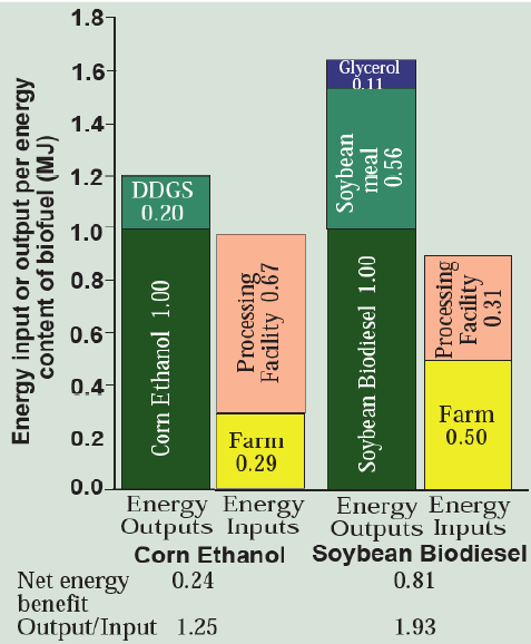
The first question to ask is: Does ethanol deliver more energy than it takes to produce? This turns out to be a difficult question to answer, though we will see that ultimately the answer is just barely. Let’s walk through a net energy analysis using Figure 8.4 adapted from an excellent 2006 study by Jason Hill and others as a visual guide. To get one unit of energy from corn ethanol, we need to use 0.29 units at the farm and 0.67 units at the processing plant. We do, however, also get 0.20 units as a by-product—distillers dry grain with solubles, a livestock feed. The net energy benefit is 0.24 units with a very low output/input ratio of 1.25. For soybean diesel, the ratio is a bit better – 1.93. So more energy comes out than goes in, but not much more. For comparison, Brazilian ethanol made from sugarcane has a ratio of about 8, several times higher. Unfortunately, we must conclude that the energy gains are meager.
Given that 18 percent of U.S. corn produced 2.4 percent of gasoline in 2006, the net gain was only 0.5 percent of the gasoline energy supply (applying the 1.25 ratio). These are discouraging numbers indeed, especially when compared with the effects of improvements in fuel efficiency. For example, with an average U.S. mpg of 21 for cars and light trucks in 2006, an improvement of only 1 mpg reduces oil use by 5 percent, ten times the net energy gain and twice the product output from all U.S. biofuel production!
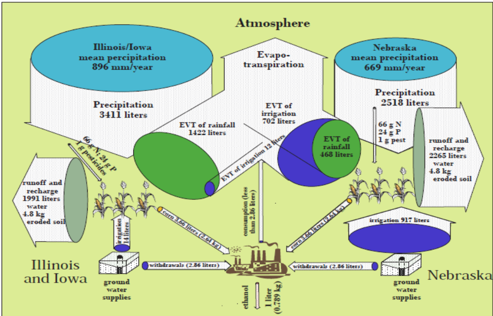
What about ethanol’s impact on other natural resources like water? My graduate student Stanley Mubako and I investigated this question using a logic similar to the net energy analysis presented above. It starts with rain falling on corn fields in Illinois and Iowa, the two largest corn-growing states, and Nebraska, the leading irrigated corn-growing state (Figure 8.5). If the corn plants transpire this water to the atmosphere, it is part of the water footprint of ethanol. This amounts to 1,422 gallons of water in Illinois and Iowa and 468 gallons in Nebraska for every gallon of ethanol produced. (Note that these volumetric ratios also apply if we prefer to use liters.)
But wait! If the fields producing the corn for ethanol plants were growing another crop or were being used for pasture or forests instead, the rain would still fall on them, and much of it would still be transpired—perhaps a little more or a little less than from the corn field. These water footprint numbers represent a huge amount of water; when applied to all the land planted to corn in these states or to all the ethanol produced in the U.S., it amounts to the entire flow of the Illinois, Des Moines, or Platte Rivers, the largest rivers in Illinois, Iowa, and Nebraska, respectively. Water transpired by rainfed corn, however, does not present a demand on scarce freshwater resources that would not otherwise occur.
If the corn acreage is irrigated, however, the water footprint does represent an additional demand. This is especially evident in Nebraska, where 60 percent of corn is irrigated, almost all from pumped groundwater, and so the 702 liters of irrigation water that transpires to the atmosphere in corn fields does represent a very large additional demand on scarce freshwater resources in competition with other uses. The amount of water used in corn fields dwarfs the use of water at ethanol plants, though this can be significant as well. This comparison of water use in rainfed vs. irrigated corn shows us that you can’t just look at the bottom line water footprint total. You also have to discern what the flows actually represent and what resource-allocation trade-offs are implicated. These same issues apply to the water footprint numbers provided in Tables 8.5 and 8.6.
From a water quality perspective, corn-based ethanol is also problematic because growing the 2.64 kg of corn needed for a liter of ethanol entails, on average, 66 grams of nitrogen and 24 grams of phosphorus as fertilizer, 1 gram of pesticides, and results in 4.6 kilograms of soil being eroded. Multiply these numbers by the liters of ethanol produced (about 20 billion in 2006) and we have a very significant water quality issue. Ethanol production is clearly a driver of polluted runoff, the leading water quality problem in the U.S. Biofuels are also the only energy source that substantially increases human appropriation of net primary production, which is in competition with food supply and biodiversity.
For better or worse, climate change currently leads the list of pressing environmental issues, and if ethanol can help, then perhaps this more than balances the meager net energy gains and high impact on land and water resources. As captured by the diagram in Figure 8.6, this appears to be the case because the carbon in oil is transferred from the earth’s crust to the atmosphere, where it contributes to climate change when it is burned as gasoline in a car. In contrast, the carbon in ethanol originally came from the atmosphere and was embedded in the corn through photosynthesis and then ethanol. When we burn the ethanol, it is recycled to the atmosphere rather than emitting greenhouse gases from the lithosphere.
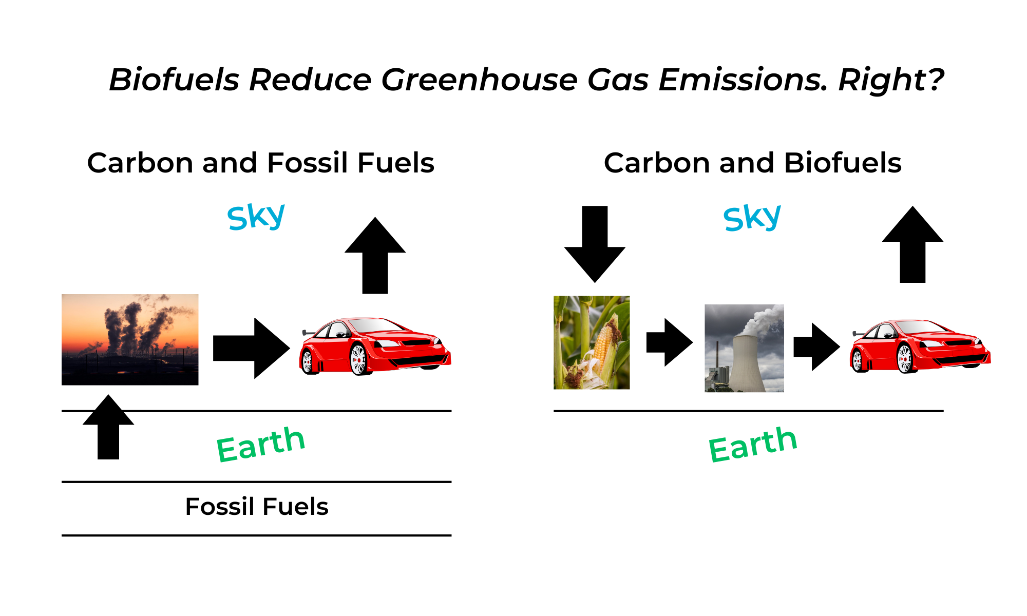
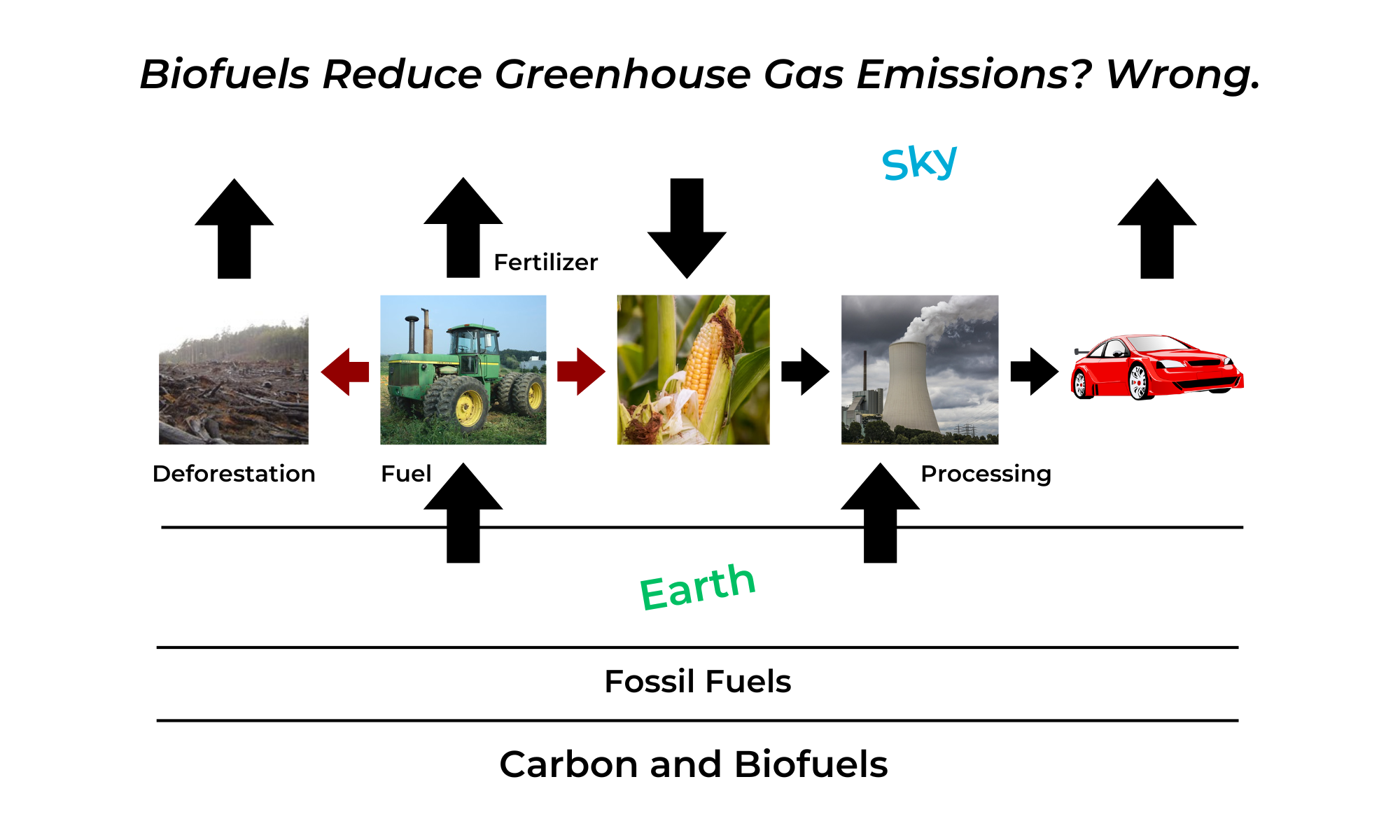
When we look closer, however, the situation changes (Figure 8.7). First, we have to include the carbon inputs of tractor fuel, fertilizer manufacture, and so forth that we examined in the net energy analysis. That leaves us with only a slight reduction in carbon emissions from biofuels as compared to gasoline from oil.
Moreover, the corn must be grown somewhere —on land that is currently used for something else. A 2008 study by Searchinger and others found that for every 5 acres devoted to corn for ethanol, 4 acres of grassland or forest are brought under crop production, largely in Brazil, China, India, or the U.S. This releases 25 percent of the soil organic carbon, plus all of the aboveground carbon in the grass and trees. Moreover, the carbon the growing forests or grasslands could have captured and stored as wood and biomass remains in the atmosphere. When this land use effect is included, ethanol ends up with twice as high a carbon footprint than gasoline over a 30-year period, and it takes 167 years for the slight improvement provided by ethanol over gasoline to restore the carbon released from the lands newly brought into crop production. So we end up with ethanol potentially exacerbating rather than ameliorating climate change.
What’s the bottom line for corn ethanol? That depends on what you value. Industrial ecology tells us that it has limited potential to replace oil imports or conserve fossil fuels, and even this is achieved at high costs to the most pressing natural resource sustainability issues we face—climate change, water resource availability, polluted runoff, meeting future food demands, and preservation of biodiversity on lands not used for agriculture. Moreover, it flies in the face of the essential macro-ecological dilemma of sustainability by placing the demands of our industrial energy supply squarely in the competition for current photosynthetic potential on this finite planet. It is HANPP.
There may be cheerier news. Ongoing research in greenhouses and laboratories shows promise of developing ethanol from more abundant plant materials that are not used for food—cellulose or algae. Most of the stalks, leaves, and wood of a plant are made of cellulose, but since humans are not ruminants like cattle and camels, we cannot digest it. Cellulosic feed stocks for ethanol production can include wheat stalks and corn stover (the cobs, leaves, and stalks) as agricultural wastes, wood wastes from lumber and paper mills, the slash left on the ground during timber harvest, or dedicated energy crops such as fast-growing switchgrass or miscanthus.
Despite optimistic prospects for the future, a very active research and development program has not yet mastered a chemical process for transforming cellulose into ethanol in a cost-effective way. Moreover, cellulosic ethanol feed stocks compete with soil conservation for organic matter or require very considerable areas of land to be dedicated to production of energy crops that may require fertilizers and irrigation.
Recent experiments using algae to produce biodiesel are intriguing. Algae is made of 50 percent oil and can potentially produce 200 times as much fuel per acre than soybeans, currently the leading biodiesel fuel stock in the U.S. The starch in algae can also be fermented into ethanol. The process requires carbon dioxide that can be recycled from power plant emissions, sludge from wastewater treatment plants, and can thrive on abundant salty ocean water. While these experiments are far from producing a commercially viable product, they show that innovative thinking may be able to produce advanced biofuels that overcome the shortcomings of corn-based ethanol revealed by this industrial ecology exercise.
Getting the U.S. Economy on a Natural Resources Diet
There are so many ideas for improving resource productivity, most of them fascinating in their own right, that I must control myself and only discuss a few at this point that exemplify how we can think more insightfully about living with a lighter footprint and be better off for it. We’ll explore more ideas specific to agriculture, forestry, water, and energy in Part III.
In 1990 Germany instituted its Green Dot system to reduce the disposal of solid waste in landfills and replace “extraction, depletion, and disposal” with “reduce, reuse, and recycle.” In addition to creating 17,000 jobs, the Green Dot program has led to the recycling of 6 million tonnes per year of what would have been trashed. In 2003 recycling rates exceeded 100 percent for paper and cardboard (161%), aluminum (128%), and tinplate (121%) as Germans used the Green Dot system to recycle additional materials not included in the program. Recycling rates for glass (99%) and plastics (97%) were also remarkably high. How was this achieved? The Green Dot system makes manufacturers responsible for the life cycle of their products, including all packaging used. This generates a backward flow of materials from homes to stores to factories and creates incentives to minimize packaging. Customers can simply return obsolete products and packaging to the stores where they were purchased. Why would they take the trouble? Because they have to buy green dots for trash bags that are not sorted for easy curbside pickup recycling.
So Germany is using economic incentives, regulations, and a life cycle approach to consumer products to drastically reduce the raw materials that have to be extracted from nature to produce and market products and the amount of consumer waste that has to be disposed of through landfills and incinerators. The system makes money and creates jobs as well, which is why so many countries are emulating it. The U.S. uses a similar system but only for tires, batteries, and few other products. Deposits on beverage containers also help achieve these objectives in states that have passed bottle bills. Think about what a Green Dot program could do for plastics pollution in the oceans.
One-third of all energy, two-thirds of all electricity, and one-fourth of all wood is used in buildings. Yet a well-designed building can reduce energy use by 90 percent by placing and constructing windows so as to make best use of daylight, optimizing heating and cooling distribution systems with local feedback and control, and other simple ideas that don’t add to construction costs.
Industrial ecology is, in many ways, the perfect complement to ecological economics. Why aren’t people just implementing all these ideas to reduce natural resource use, invest in natural capital, and produce ecosystem services? It’s all in the carrots and sticks. And to better understand that, we turn to institutional economics.
Additional Reading
Fischer-Kowalski, M., 1999. Society’s metabolism: The intellectual history of materials flow analysis, Part II 1970–1998, Journal of Industrial Ecology 2(4):107–136.
Haberl, H., K-H Erb, F. Krausmann, 2014. Human appropriation of net primiary productivity: Patterns, trends, and planetary boundaries. Annual Review of Environmant and Resources 39: 363-91.
Haberl, H., Fischer-Kowalski, M., Krausmann, F. and Winiwarter, V. (Eds.), 2017. Social Ecology: Society-Nature Relations across Time and Space. Springer.
Hoekstra, AY, Chapagain, AK, 2011 . Globalization of Water: Sharing the planet’s freshwater resources. Blackwell, Oxford.
Media Attributions |
|
