Like fire, people are mesmerized by water. A babbling brook, a placid tree-lined lake, the foam of crashing waves on the seashore—people can’t take their eyes off it. Water is my favorite resource to study because it intersects closely with other important resources like land and agriculture as well as energy, while it is, at the same time, a critical part of the environment, even if the “life blood” metaphor has become hackneyed. We have already taken a look at the hydrologic cycle in Chapter 3. Here we will study how humans utilize water, especially the small proportion of it that is fresh rather than salt, and how it can be used sustainably.

In the resource taxonomy illustrated in Chapter 7 and Figure 7.6, water is a flow resource. The hydrologic cycle is driven by solar energy, which is perpetual; as long as the sun shines, water will continue to be evaporated and distilled from the ocean, transported over land, and fall as precipitation, the fundamental form of freshwater resource available to a region. That’s the good news. Precipitation is less reliable than sunshine or even wind, however, and this raises the issue of storing water from prior precipitation for later use. The slowly melting snowpack on a mountain range serves this purpose admirably for free. The water flowing quickly to the sea in streams and rivers usually represents precipitation that fell in the last week or month. The soil also stores water for weeks to months for crops and other plants as we saw in Chapter 3. The water in a reservoir formed by a dam on that river or a natural lake may contain somewhat older precipitation on the order of years. Groundwater, on the other hand, may be water that originally fell as rain centuries, even millennia, in the past. If an aquifer recharges every year from infiltration and percolation, then we can still think of it as a renewable reservoir, but if the recharge rate is slower than the rate at which it is pumped, water can be as nonrenewable as oil. The water itself is not destroyed when it is pumped and applied, say, as irrigation for crops, but it re-enters the hydrologic cycle either by evaporating or transpiring to fall as rain, likely on the salty sea, or runs rapidly down rivers to the same destination. It is in this sense that the measure of water consumption is evapotranspiration.

As a natural resource, then, fresh water is similar in some ways to forests, which we discussed in Chapter 11. It is renewable but only at a finite and variable rate defined by natural processes. For this reason, we need to carefully manage the limited reservoir available for future use, just as we do the stock of standing timber. Also like forests, which can be destroyed by fire or land clearing, the usefulness of water can be destroyed by pollution. While water does not reproduce biologically like forests, fossil groundwater is as irreplaceable as ancient redwoods and sequoias—on a human time scale, these are stock resources. Unlike forests, however, water can sometimes be overabundant. Among natural hazards, flooding is the leading cause of property damage, even though earthquakes can claim more lives.

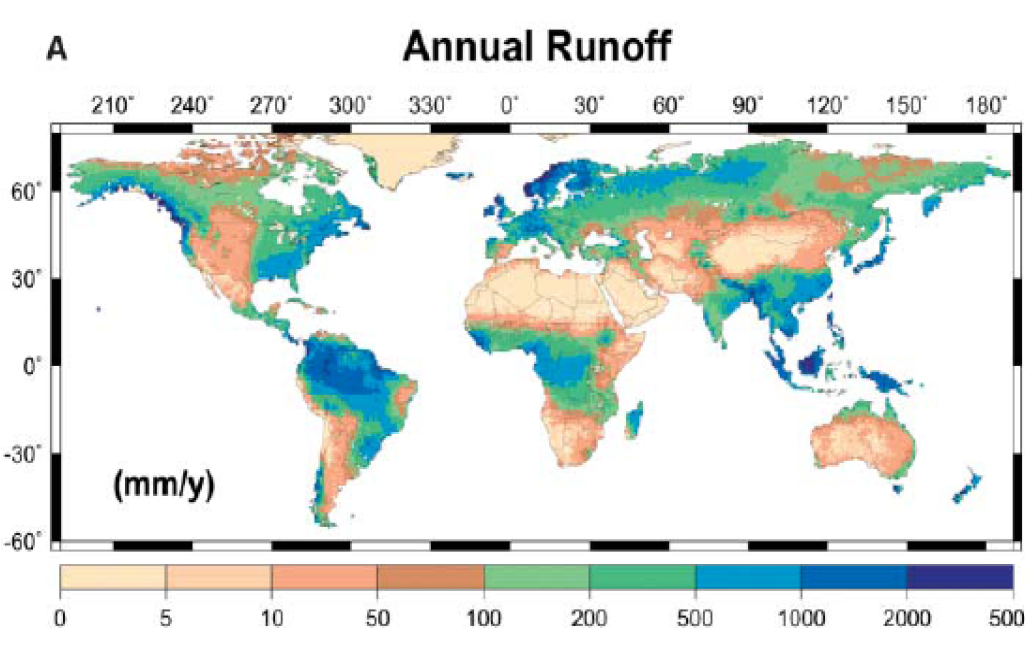
On average, freshwater is relatively abundant but on average doesn’t help us much more than you having enough oxygen to breath on average. Figure 12.1, repeated from Chapter 3, demonstrates the great geographic variation in freshwater runoff from precipitation—the part of the hydrologic cycle that can be captured by humans and put to work. Note again that the scale in millimeters per year is logarithmic, meaning that the areas in dark blue have 1,000 times as much water as the areas in light tan. It is again worth pointing out that nearly the entire human race lives in areas with between 50-1,000 mm/y (about 2–40 inches) of annual runoff. You could rebut that the blue areas with surplus runoff of over 1,000 mm/y could give the extra water to the brown areas with less than, say 100 mm/y. Massive transportation of water rarely works out, however, because, even in the 21st century, rivers can’t be rerouted in a practical manner (with a few amazing exceptions and grandiose plans, such as one to reroute much of the flow of the Yangtze River in China north to the desiccated Yellow). As a bulky, heavy substance with a low value per unit weight, it is not economical to transport huge quantities of water long distances. So water resources are tied to specific geographical areas usually defined by watersheds.

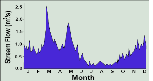
The availability of freshwater also varies greatly over time. Repeating the hydrograph shown in Figure 3.4 as Figure 12.2 shows the flow of a stream varying 26-fold. In arid regions, stream flow varies even more, from nothing most of the time to deadly torrents upon occasion. Storing these torrents behind dams for later use can be very helpful, but reservoirs encourage losses to evaporation and can run dry during extended droughts. Getting the right amount of water at the right quality to the right use in the right place at the right time is the ever-present dilemma in water resources management.

How Humans Use Water

Go ahead, take a drink; that’s the most fundamental, and the most important, use of water because, well, it keeps us alive. But it isn’t even the tip of the iceberg of human uses of water. Let’s begin with what likely comes to mind next, after drinking—the use of water in homes and buildings in such everyday ways as the kitchen faucet for cooking and cleaning, the bathroom for showering and the toilet, and water-using appliances such as dishwashers and clothes washing machines. The average American uses 30 gallons per day in this manner, the most of any country, though it has declined considerably due to efficiency improvements. Add in outdoor water uses, mostly from the hose nozzle—watering the lawn and garden, filling the swimming pool, washing the car, even clearing the sidewalk—and we’re up to 59 gallons per person per day, though the regional and seasonal variation of outdoor uses is much greater than for more essential indoor uses.

Now let’s consider commercial water use—water fountains and restrooms in schools and other public buildings, restaurant kitchens, hospitals, and so forth. Then we add in industrial water used in light manufacturing plus outdoor water use in all these to keep that nice green grass and shrubbery look that attracts customers and makes things look legit.

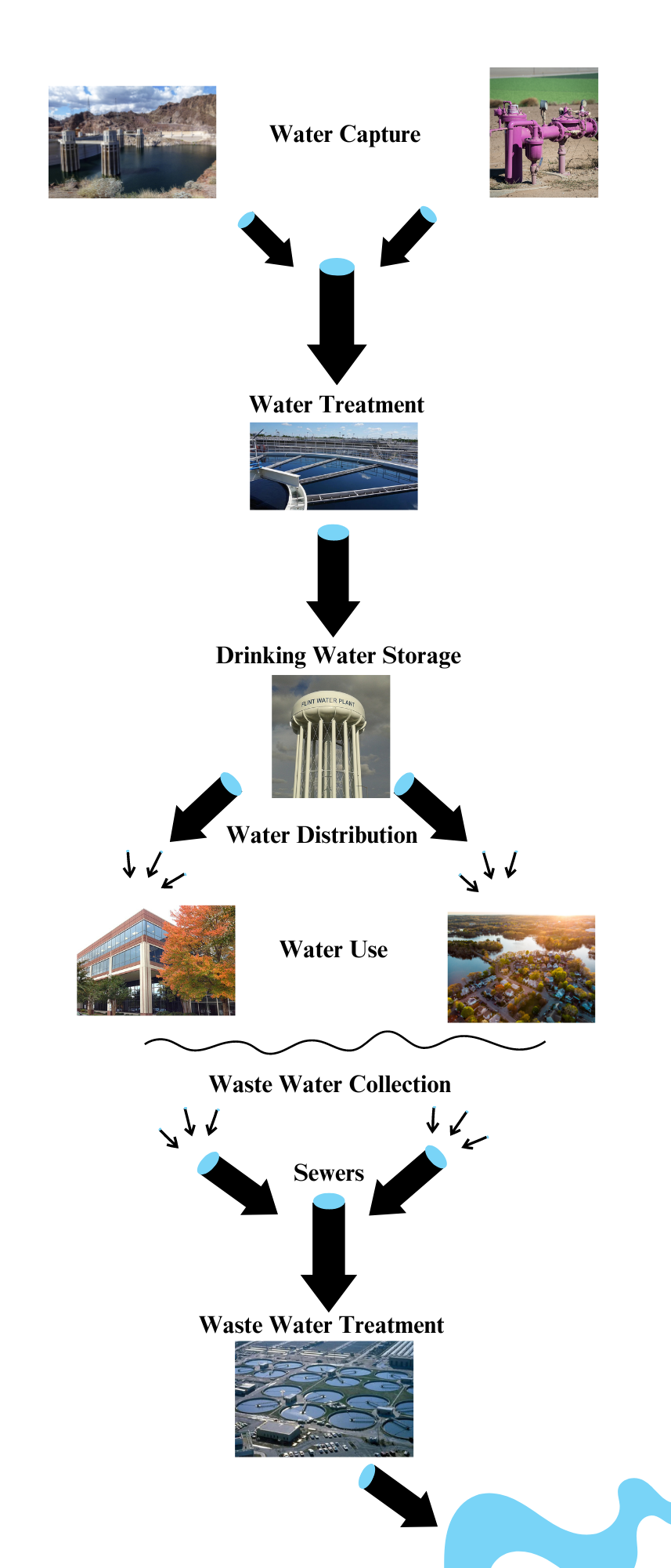
In most cases, all of these uses are supplied by municipal water supply systems, one of the most fundamental and critical infrastructures that makes modern life possible. Figure 12.3 diagrams the essential elements in a municipal water supply system. First comes the capturing of water from a natural source: wells for groundwater and usually dams to store the erratic flows of surface water in reservoirs. The water is then piped to the water treatment plant where raw water is purified according to the specifications of the Safe Drinking Water Act. Chlorine is added to kill algae, bacteria and viruses that are always present in water, even in pristine wilderness brooks. A flocculent is also sometimes added to get the suspended clay particles to coalesce and sink to the bottom, clarifying the water.

By and large, public water supplies in the U.S. are safe to drink, at least as safe as expensive bottled water, though problems can arise, especially from trace chemicals that can very slightly increase the risk of cancer and other health problems. The last major outbreaks of waterborne illness in the U.S. occurred in Milwaukee in 1993 when cryptosporidium, a form of bacteria from livestock manure, infected the public water supply, sickening 403,000 people and killing over 100. In 2014 Flint, Michigan switched its water supply from Lake Huron to the Flint River and failed to add chemicals needed to prevent it from leaching lead from the interior of old pipes. As was reported in the national news, over 100,000 residents, many of them children, suffered from lead poisoning, whose effects on their nervous systems may be lifelong. Many think Flint is the tip of an iceberg made of old lead pipes.

Here’s where the water supply system gets really interesting from an engineering standpoint. Consider the circulatory system in your body, starting at your beating heart, which provides pressure. Blood rushes from the heart through the aorta, then through arteries to innumerable capillaries. Similarly, the water tower or mountainside reservoir, being higher in elevation than the faucets, provides pressure to connected water mains and smaller pipes to every faucet, shower, and toilet in the city—hundreds of thousands of them in even a small city. When you open the tap, water is forced out by gravity manifested as hydrostatic pressure. Moreover, dirty, untreated water can’t get into the piping system because the pressure pushes it out. This ingenious system for delivering high-quality water to an entire town or city was invented by the Romans for their capital city with its famous ancient aqueducts and is now used worldwide in various forms. At least one billion people do not have access to treated, piped water, however, a humanitarian and development issue we will explore below.

Once the water is used, there is a physically separated wastewater system analogous to the veins that lead back to the heart. Water goes down the drain or toilet to the wastewater system. In urbanized contexts, the wastewater pipes from homes and buildings funnel into sewers which feed downhill to the wastewater treatment plant. At the plant, primary treatment screens and filters the water to remove large objects which are then land-filled or incinerated. The remaining water undergoes secondary treatment where activated sludge—bacteria whose reproduction is stimulated by extra oxygen—essentially eat up organic matter in the water. The fertile, but possibly contaminated, sludge is used in land reclamation, such as on coal-mined lands or to establish golf courses. It can also be used to grow algae for biofuels.

In most cases, the water is then released to nature—usually a stream or river, but sometimes a lake or the ocean. In other cases, it undergoes tertiary treatment, sometimes in natural or created wetlands or in sandy filters leading to aquifers, where nutrients (N, P) and other pollutants are reduced. The resulting water is not fit to drink, though it is possible to feed it into the drinking water plant in a recycling system. Most people are a bit “woozy,” however, about drinking recycled sewage. Even if the wastewater treatment plant outflow is not fed into the drinking water treatment plant directly, reclaimed wastewater can still be put to industrial, agricultural, or landscaping uses. In arid regions, this is an important part of the non-potable water supply of cities. As small, separate wastewater systems, many rural homes and buildings use septic tanks and drainage fields to seep the water back to nature after bacteria eat up most of the nasty organic wastes.

Because cities have so much impervious surface—roofs, roads, and parking lots where rain runs right off without infiltrating to groundwater or transpiring—they also require stormwater systems. We often see these as gaps under the curb in low-lying areas along the street where the rainwater seems to disappear down the storm drain. In many cities these stormwater systems join with the sewer lines to end up at the wastewater treatment plant. During a heavy rainstorm, however, the plants can be overwhelmed with water and the sewage can pass through untreated. In other cities, the stormwater system empties directly into a stream, river, lake, or the ocean untreated. Some cities are beginning to use a more green approach, feeding storm water into wetlands and ponds where nature can begin a purification process while encouraging infiltration and evapotranspiration. Others are using pervious pavements in parking lots so the water can infiltrate rather than run straight down to streams to generate an urban flash flood. As is often the case with natural resource management problems, stormwater management seems mundane, but it is an important wrinkle in sustainable water resource management, and intensifying rainfall events due to climate change are making it even more essential.

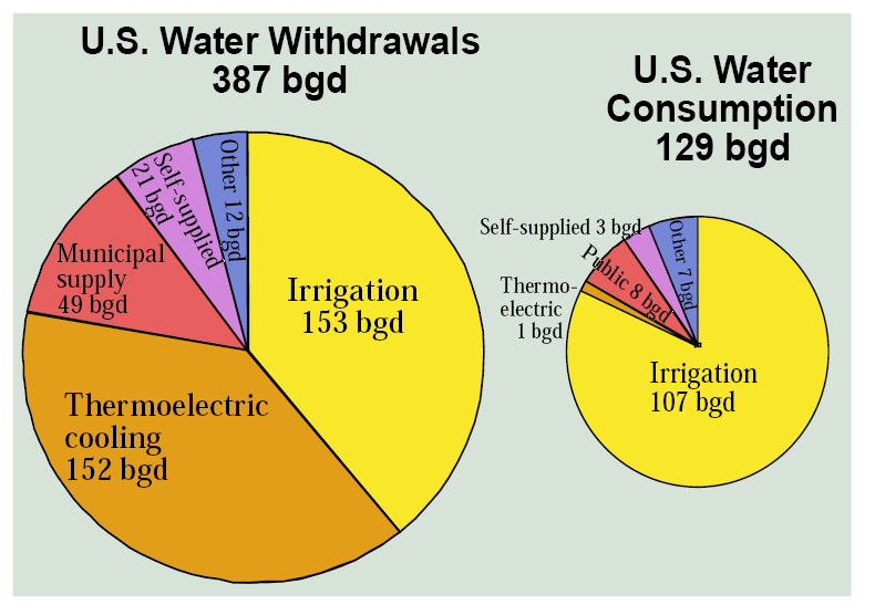
We’ve now discussed a lot of uses of water, but we’re still only getting started. Large industrial facilities like paper mills and food processing plants usually have separate water systems not hooked into the municipal supply system. Thermoelectric (coal, gas, and nuclear) power plants are especially large users of water for cooling. In the U.S., withdrawals of water for this purpose are three times higher than for all municipal supply purposes put together. Power plants are neck-and-neck with irrigation as the largest source of U.S. water withdrawals (Figure 12.4). In fact, power plants are built adjacent to water supplies rather than fuel supplies to minimize the distance huge quantities of water have to be pumped and piped. Fortunately, salt water serves as well as far more scarce fresh water for this purpose, explaining why many power plants are built along the coast. Before 1960, 80 percent of power plants built once-through cooling systems where about 99 percent of the water returns to its source—several degrees warmer. Since 1980, 80 percent have constructed cooling towers; these reduce water withdrawals by up to 95 percent but result in much more loss through evaporation. If we also consider the water passing through hydroelectric dams and evaporating from their reservoirs, as well as water needed to produce biofuels and fossil fuels, it is clear that much of the water we use goes to produce our energy supply. This is often called the water-energy nexus and it also includes the energy needed to pump and treat water.

We’ve still only covered the tip of the iceberg, however, because food production is the largest use of water. This comes in two primary forms: irrigation and rainfed agriculture. Irrigation is the deliberate application of water to plants, especially crops, to encourage their growth. In arid and semiarid regions, irrigation is required to make crops grow, though water resources are limited. In wetter climates, supplemental irrigation can counteract the effects of drought. In the U.S., irrigation is roughly tied with thermoelectric cooling in withdrawals but leads in withdrawals of fresh water since salt water kills crops. Because most thermoelectric withdrawals are quickly returned to the source, irrigation is by far the leading source of water consumption, with 83 percent of the U.S. total of 129 billion gallons per day (bgd) (Figure 12.4). This is even more the case globally; 87 percent of water consumption is for irrigation.

All of the human uses described above require water to be withdrawn (i.e., pumped) from a natural source—a reservoir, lake, river, or aquifer. When human water uses are characterized and measured, such as by the U.S. Geological Survey, we measure water withdrawals; these total 387 billion gallons per day (Figure 12.4) for the U.S. The second measure is water consumption—the amount of water that evaporate or transpires away into the atmospheric component of the hydrologic cycle. Swedish scholar Malin Falkenmark makes the case that this presents only a partial view of water use, what she terms blue water. First, if food production is the dominant use of water, why count water applied to crops as irrigation and not also count water that falls as rain on crops? Rainwater, which is drawn from the soil and transpired by crops as an essential element in their growth, is called green water. Green water use in the U.S. has been estimated at 357 bgd, nearly as much as all withdrawals and about three times higher than all other sources of water consumption. Factoring in green water drives home the point that the dominant human use of water is agriculture, and it explodes the average American’s daily water use to 1,794 gallons.

Table 12.1 shows how much water it takes to produce a variety of everyday items and common agricultural products. (Remember that a liter is very close to a quart or a fourth of a gallon and weighs a kilogram, 2.2 pounds.) The primary reason these numbers are so high is the huge amount of water that is transpired by crops, including those eaten by livestock. So the majority of the water content in the products listed in Table 12.1 is green water, rain used by crops, rather than blue water withdrawn from natural sources.

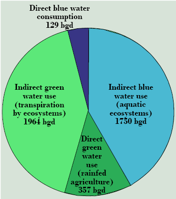
We’ve now covered human uses of water for provisioning ecosystem services as a factor of production in the economy, but what about supporting, cultural, and regulatory services, all of which require water? We’ll term this indirect water use. Indirect green water use of 1,964 bgd is transpired by natural ecosystems—forests, wetlands, and grasslands. When we benefit from the services these ecosystem provide, we are indirectly using the precipitation that fell on them and was then transpired back to the atmosphere. Indirect blue water use of 1,750 bgd is precipitation that flows into lakes, streams, rivers, and on down to the ocean, making aquatic ecosystems—and the services they provide—possible. These include hydroelectricity, navigation, fishing, recreation (in-stream uses), nutrient cycling, maintenance of biodiversity, and just gazing at it – a luxury that places a substantial premium on waterside homes. So, in one way or the other, we use the entire endowment of 4,200 bgd of precipitation that falls on the United States annually (Figure 12.5).

It is encouraging that blue water consumption is, for the U.S. as a whole, only about three percent of the rain and snow that falls from the sky. That number is also not very meaningful or helpful, however. To see why, let’s explore perhaps the most scenic river basin in the U.S.—the Colorado River, author of the Grand Canyon.

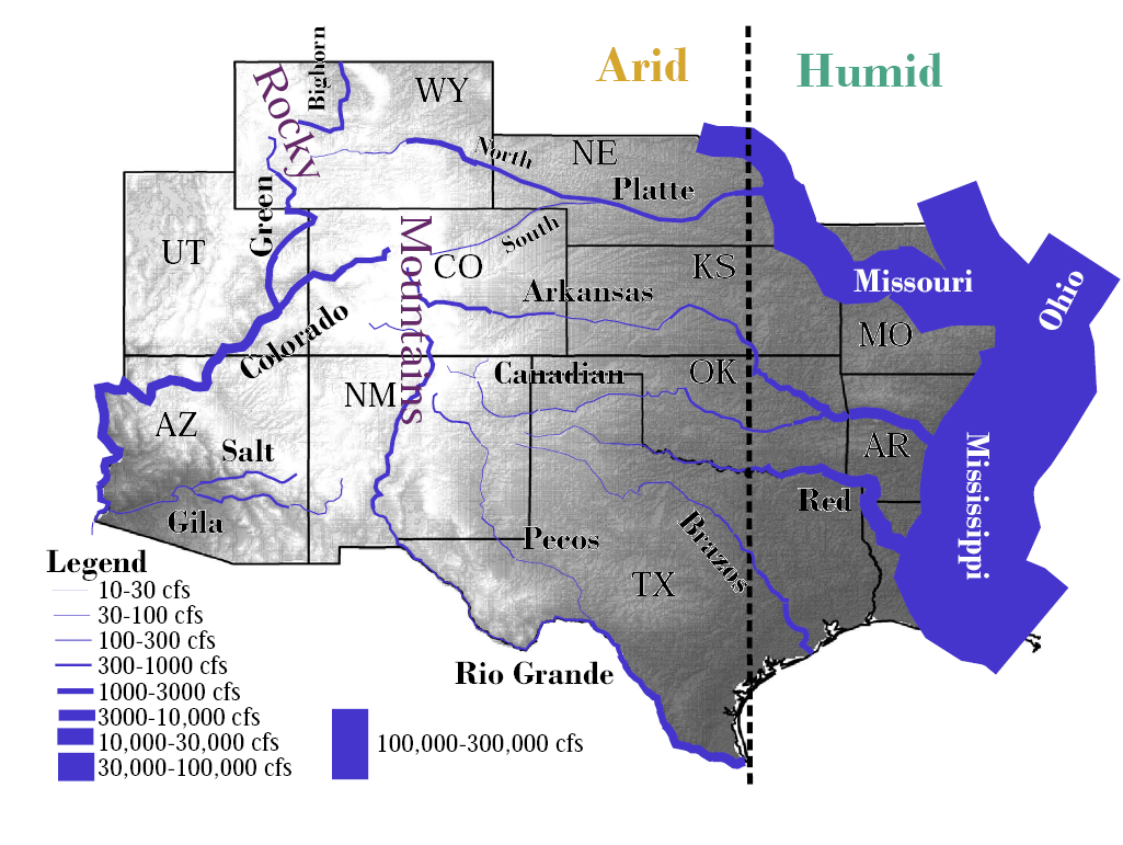
The Colorado River (Figure 12.6) runs from the Continental Divide in the Colorado Rockies westward, where it joins the Green River—flowing south from southwestern Wyoming—in eastern Utah at Canyonlands National Park. Flowing southwest, the Glen Canyon Dam at the Utah-Arizona border forms Lake Powell, the terminus of the upper basin. It then bends west, enters the Grand Canyon (a marvel you simply must see despite the crowds from all over the world) reaching Lake Mead, held back by the Hoover Dam along the Nevada border. From there, the river heads south to form the Arizona-California border until it crosses into Mexico and ends its 1,450 mile journey at the Gulf of California.

Except that the Colorado does not end there because only rarely does any water reach the Gulf. The rest is used, and consumed, along the way by irrigation farmers—from Wyoming to southern California—and by Las Vegas, Phoenix, Tucson, Los Angeles, San Diego, and other cities, all of whom pipe water uphill from the Colorado River. Some water is even tunneled beneath the Continental Divide to the cities of the Colorado Front Range and beneath the Wasatch range to Salt Lake City in interbasin transfers. The river ends in a thousand irrigated fields and dozens of water treatment plants. It’s used up. The delta, once perhaps the most vibrant ecosystem in the region, is barren desert.

The Colorado is not alone in this fate (Figure 12.6). The Rio Grande brings water from the Sangre De Cristo Range in southern Colorado to Albuquerque and El Paso as well as irrigation farmers in the valley—then dries up. The Rio Grande then re-emerges further east where its tributary, the Rio Conchos. arrives from Mexico.

The Arkansas River flows east from the Sangre de Cristo, but it barely enters Kansas before it runs dry, only to reappear in eastern Kansas where rainfall is great enough to produce perennial streams. It’s not just surface water that is being consumed. Recall from Chapter 2 that water tables in the Ogallala Aquifer are dropping from western Kansas to north Texas. The same is occurring in parts of California where the land is subsiding above dewatered aquifers. Most of the southwestern United States is using all its available water, and climate models predict the region to grow considerably drier. This is the region—the Sunbelt—that Americans are flocking to!

It is no consolation that the Great Lakes are the world’s second greatest storehouse of liquid, fresh water (mile-deep Lake Baikal in Russia is first) or that the Mississippi is the most voluminous river in North America. Even if the states possessing these vast resources were to allow it to be exported, which they will never do, the cost of engineering schemes to transport the water would be in the tens to hundreds of billions of dollars. For California, desalinating ocean water is an option, but an expensive and energy-intensive one that only the affluent city of Santa Barbara has taken, and they regret the expenditure. At a cost of $0.50–$1.00 per cubic meter, or about $600–$1,200 per acre-foot, desalinated water is not cost competitive with leasing water from irrigators and is too expensive for use in agriculture.

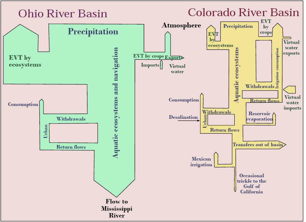
One way of integrating these issues for a specific river basin, and comparing it to others, is through a water flow diagram such as shown in Figure 12.7. On the left, a prominent eastern river basin, the Ohio, averages over 40″ of annual precipitation. There is almost no irrigation in the basin, though rainfed agriculture is important. The basin exports more virtual water than it imports (we’ll explore the concept of virtual water below). The greatest source of withdrawals is for thermoelectric cooling with high rates of return flow. The Ohio and its tributaries support abundant aquatic ecosystems beneath the high volume of barge traffic. Huge quantities of water discharge to the Mississippi, of which it is the largest tributary.

Using the same technique, the somewhat larger Colorado River watershed appears very different. Far more scant precipitation is transpired by ecosystems, withdrawn and consumed by irrigation, evaporates from reservoirs, is transferred out of the basin, or is consumed by urban and industrial uses. The small volume reaching Mexico is consumed for irrigation there, leaving only an occasional trickle of water to reach the Gulf of California. The basin imports more virtual water than it exports, and it utilizes small quantities of expensive desalinated water. Water managers consider removing scant riparian vegetation to conserve water transpired by ecosystems. No water is left unspoken for; an increase in any water use implies a decrease in some other use.

With your mind’s eye, you can perhaps imagine these diagrams in motion, expanding following snowmelt and rainstorms and contracting during droughts. A similar water use flow diagram could be developed for any river basin, and comparing them would reveal a great deal about the water resources challenges they face.

The answers for the Colorado and other river basins in the American Southwest do not lie in increasing water supplies; they must lie elsewhere. One option, of course, is water conservation or demand management. Low-flow toilets, shower-heads, and “water sense” appliances make a big difference if the majority of the population is employing them. These nonconsumptive water uses deliver water to the wastewater system, however, where it can potentially be recycled. An even bigger dent can be made through xeriscaping—replacing the green grass, shrubbery, and big shade tree look with attractive, desert-like landscaping that requires several times less water. Through these and other techniques, municipal water use has fallen from 100 gallons per capita per day in the 1990s to 59 in 2017, an enormous accomplishment in improving water use efficiency, even though the water mains in many older cities are over a century old and leak chronically.

Water can be harvested in barrels and cisterns from occasional rains falling on the roof. Better yet is using aquifers, which are not open to evaporative losses, rather than surface reservoirs for water supply storage. Increasing the price of water reduces the amount used, especially if prices per gallon increase as more gallons are used.

We must remember that conservation, reductions in use, must come from where the water is now going—predominantly agriculture. It also makes more sense to conserve on less valuable and more consumptive uses of water such as irrigation rather than more valuable and less consumptive uses occurring indoors. Irrigation efficiency, a topic that at first seems mundane, suddenly rises toward the top of the list in water resource sustainability. It’s time to start talking about acre-feet—the amount of water needed to cover one acre of cropland one foot deep in water: 325,851 gallons.

There are a number of levels of irrigation efficiency. The first is “more crop for the drop.” Flooding an uneven field from an unlined ditch does work—farmers have been doing it for thousands of years—but it is not an efficient approach to maximizing the bushels produced per acre-foot of water applied. Overhead sprinklers are not only more efficient, but the commonly-used central-pivot system makes lovely circles on the landscape that amaze airline passengers gazing out window seats as they traverse the Great Plains. More efficient yet is drip irrigation where small, perforated pipes in the soil deliver water, sometimes with fertilizer mixed in, directly to crop roots one drop at a time. As water use efficiency goes up, however, so does the cost of investing in irrigation equipment. This can only be paid for with the value of the water conserved. Water is generally subsidized and underpriced, or even free, even in arid regions, undermining the economic incentives needed to encourage purchase and installation of efficient irrigation equipment. As we concluded in Chapter 6 on neoclassical economics, “that which is cheap gets wasted; that which is expensive gets conserved.”

The second level of irrigation efficiency could be called “crops that drink fewer drops.” Table 12.2 shows typical amounts of water used per acre for a variety of crops, typical yields per acre, and typical revenues by multiplying by price. Dividing the revenue by the water use produces a measure of economic value per unit of water applied. We can clearly see that water used to irrigate pastures or grow alfalfa for cattle produces little revenue. It’s not the highest and best use. Drip irrigation on vegetables produces many more dollars per acre-foot. Economics would dictate that scarce resources be reallocated from lower-value to higher-value uses. A higher price for water would also make low value uses uneconomic. For example, at a price of $100 per acre-foot, irrigating pasture, alfalfa, and rice produces an economic loss. This price would reallocate water now used for these crops to other more valuable uses, not only corn, soybean, and vegetable production but municipal water supplies, and possibly leaving the water in the stream to support fish and other aquatic life, though it is very difficult to measure a per acre-foot dollar value to aquatic ecosystem services.

The third level of irrigation efficiency is called virtual water, but “virtual” anything always requires an explanation. Let’s say southern California phases out irrigation of 10,000 acres of corn, saving 30,000 acre-feet of water, half for environmental uses like in-stream flow, and half for urban uses where the 15,000 acre-feet are worth $10,500,000. Instead they import or buy the 60,000 tons of corn the irrigation would have produced from Iowa for $3,600,000, saving $6,900,000 with improved aquatic ecosystems as a bonus. This corn required 30,000 acre-feet of rain falling in Iowa to grow and was sent to California on a train instead of being sent to an ethanol plant. In an important sense, southern California is gaining access to these 30,000 acre-feet of Iowa rain and coming out ahead because the urban and environmental uses of the water are more valuable to California than the corn it is no longer producing. It is also a better solution than transporting the 41 million tons of water from Iowa because the corn weighs only about 41 thousand tons, 1,000 times less, than the water used to grow it. Iowa also benefits by gaining an additional export market for their abundant harvest of rainfed corn. In this way, water-surplus regions can make money by selling water-intensive products like crops and livestock to water-deficit regions. This allows the latter to reallocate their scarce water supplies away from consumptive, low-value irrigation to less-consumptive, higher-value urban and environmental uses.

Virtual water is an example of what economists call comparative advantage. Regions are better off using their best endowments to produce a surplus for export while importing goods and services for which they lack resources. It runs against the notion of local self-sufficiency, however, and therein lies a few caveats. Using the virtual water strategy makes arid regions dependent on humid regions for their food supply and undermines local agricultural economies. Now only the most paranoid person would worry that Iowans are going to embargo food from Californians, but on a global scale, food security is a limitation on virtual water trade. The Middle East is the world’s most water-deficit region and North America the greatest exporter of virtual water. Would that region trust North Americans with their essential food supply any more than Americans trust Middle Eastern countries with their essential oil supply? In fact, they do.

A 2004 global study of virtual water trade by UNESCO shows some fascinating patterns (Table 12.3). The U.S. exports 131 bgd, about the same as total withdrawals or the flow of the Ohio River, with net exports of 108 bgd. North America is by far the leading virtual water exporting region at 162 bgd with net exports of 149 bgd. South America (35 bgd), Oceania (22 bgd) Southeast Asia (20 bgd), former Soviet Union (7 bgd), Central America (4 bgd), and Eastern Europe (1 bgd) are also net exporters. The leading net importing region is Central and South Asia at 120 bgd, followed by Western Europe (56 bdg), North Africa (32 bgd), Middle East (22 bgd), Southern Africa (3 bgd), and Central Africa (1 bgd).

What underlies these patterns? Virtual water net importing regions are those that struggle for food self-sufficiency either because they lack rainfall (North Africa, Middle East, Southern Africa, part of South and Central Asia) or they are very densely populated (South Asia) or both densely populated and affluent enough to afford huge supplies of food and raw material imports (Western Europe). Net exporting regions have modest population densities relative to their endowment of crop-producing soil and rainfall (e.g., South and North America). Through virtual water, the New World feeds, and thereby indirectly waters, the Old. In a similar manner, can the Eastern U.S. water the Western U.S. by selling it food, cotton, lumber, paper, and other water-intensive products? This would reallocate scarce western water from low-value irrigation to higher value urban uses as neoclassical economics would indicate and to ecosystem service provision as ecological economics would indicate. To unravel why these seemingly sensible schemes to reallocate western water are not as straightforward as one might wish, we need to take a journey into the dilemma of prior appropriation, the legal system for allocating the use of water in the western states.

The Dilemma of Prior Appropriation

Imagine yourself as a pioneer in the mid-1800s heading west to the lands the U.S. bought from Napoleon (the Louisiana Purchase), more recently split with British Canada (the Oregon Territory), annexed from the Mexicans (the Southwest), or took from the Native Americans (all of the above). The U.S. government is encouraging you to go because, if these vast lands are not occupied quickly, they could be lost to their former owners. The mountains and canyons are breathtaking but, as the explorer John Wesley Powell pointed out again and again to anyone who would listen, the land is too arid to support the standard homesteader approach of establishing a rainfed farm on a few hundred acres.

Given this limitation, your first option for establishing a livelihood is mining, especially for that pretty yellow metal that’s worth a lot of money. The best way to get at it is through hydraulic mining—blasting the streamsides with a fire hose to release the rock and sediments. Then you’re ready to pan for gold. Your second option is farming to feed all those miners, but this requires irrigation. Either way, you need water and there’s not much of it to go around. So you establish a mining operation by diverting water from a stream and you have enough success to make a living in this grand new country where the sky is not cloudy all day.

A decade later, another party of pioneers arrives and, seeing how success in this dry country depends on access to water, settle upstream of you so they can divert the stream for an irrigated farm. But that leaves you without enough water to continue mining. Rather than challenging them to a duel, you decide to take a safer route and call upon the county judge. Smart move, because the judge decides “first in time, first in right.” The prior appropriation of water—your senior and continuing mining operation—has precedence over junior (more recent) appropriations of water. The judge orders the newcomers to cease and desist in diverting water from the stream to their farm. Subsequent cases use this precedent, western states pass statutes codifying the system, and prior appropriation is established.

In this hypothetical case, the judge was right. If he had decided in favor of the late-coming irrigators, new pioneers could simply leapfrog one another up the valley to get at the water upstream of earlier users, in the process inciting innumerable conflicts. Moreover, by protecting your right to use the water in your mining operation, you are rewarded for heading west early, despite the hardships of the frontier, with a perpetual right to use water that your heirs can inherit. You have helped establish an economically viable American presence on the land, so long as you keep putting that water to a beneficial use and don’t move on or give up mining to become a guitar player or a judge. Use it or lose it. Not every valley has gold, however, and in other valleys, irrigation farmers and ranchers made first claim to most of the water.

Now let’s fast-forward to 2020. Los Angeles is the second biggest city in the country and California is the most populous state. Denver, Las Vegas, Phoenix, Sacramento, Salt Lake, San Diego, and San Francisco-Oakland-San Jose are big enough to have pro sports teams. Albuquerque, El Paso, and Tucson may soon get there as well. These cities want the water the old pioneers have locked up in farming and obsolete mining operations, and they’re willing to buy it at prices ranging from $300–$800 per acre-foot that would be difficult to refuse (see Table 12.2). Environmental groups are also making offers to leave the water in the river to protect endangered fish species. Sporting groups are making offers to improve dynamite trout streams and white-water rafting rivers. But little water gets sold from lower to higher value uses. Why?

That’s a terribly complicated and frustrating question to answer, but I’ll take a stab at it, even if I’m not a lawyer. First, you have to own something before you can sell it. The pioneers’ heirs don’t own the water any more than I own my office at Utah State University. The state owns the water and Utah State owns my office. They, and I, have a right to use it, for a specific purpose, so long as we keep using it for that purpose. (Writing this text qualifies as a beneficial use of my office!) These are usufructuary rights, not real property. Second, did anybody ever go to the state engineer’s office and write it all down? Where? When? For what use? Using what method? With what result? Third, how much water are we talking about? 62.384 acre-feet per year? Unless the watershed has been adjudicated—an expensive process of identifying and quantifying all the water rights in a river basin—nobody has ever accurately measured it. So how can I sell something I really don’t own and I don’t know how much of it there is? Moreover, like my office, if I try to sell it, that just shows that I’m not using it anymore and the state will give it away to the next person in line—a junior appropriator—just like my department will give my office to someone who can make better use of it if I stop writing and teaching.

Fourth, water flows down streams to rivers to the sea (or an interior basin like Great Salt Lake). Where is the buyer relative to the seller in this system? Is there a third party in between whose water rights would be harmed by a transfer? Fifth, what if someone invents a better way to mine gold that uses a lot less water? If I adopt it, I lose my water right. The same is true for farmers who are contemplating more efficient irrigation practices or giving up on something as wasteful as watering pastures to raise of few extra cows. Neither has any more incentive to conserve than I have to use only half my office. And leaving the water in the stream for fish is not on the list of beneficial uses. I guess that old 19th century judge never took ecological economics and learned about ecosystem services. We’re in one heck of a legal mess here but this problem illustrates how important the institutional economic approach, which examines how the law structures carrots and sticks, can be.

Some western states, especially California, are making progress through the legal minefield of prior appropriation. In the droughts of the 1990s, they established water banks. Very few people who have a right to use water in perpetuity are willing to give that up, so the focus is on leasing the right for a season rather than selling the right permanently. Second, rather than individuals buying and selling to each other, the state engineer serves as the clearinghouse. Those pioneers’ heirs can lease mining and irrigation water to the state for a rental fee—say $200–$400 per acre-foot—and the cities buy them up. The state keeps a small portion of the water to leave in the streams (a water tax) and does a complex geographical and hydraulic analysis to determine how best to move the water from all the sellers to all the buyers along existing streams, rivers, canals, and pipelines. Since the state is the buyer, sellers are immune to the use it or lose it snag. Water banking can work in other western states as well.

With southwestern cities growing in population relentlessly, with no undeveloped water around to increase supplies, with enough water to maintain habitat for endangered species of fish required by law, with climate change making the Southwest ever drier and melting the mountain snows earlier in the spring, water banking and similar quasi-market arrangements for reallocating water must work. The future of the American West depends upon conserving and reallocating its increasingly scarce freshwater resources in a sustainable manner, and water conservation and reallocation is the only sustainable approach.

Now combine water reallocation with virtual water. Let’s say dry western states import more basic food commodities like corn, soybeans, wheat, and hay from the Midwest, where these crops are in surplus and grown using green water. This could come, for example, from corn now destined for biofuels. Western farmers then lease or sell some of their water rights to cities and for environmental purposes at a profit. By taking greater advantage of these regional comparative advantages, the Western prior appropriation states greatly alleviate their water scarcity problems. Virtual water becomes real water through trade and reallocation. Is this a sustainable solution? I think it’s the best idea now on the table.

The Water Simulation

Based on prior appropriation rules and set in the New Mexico section of the Rio Grande Basin, the water simulation serves well as a classroom exercise and/or an individual assignment. Figure 12.8 shows the simulation user interface. The game is initiated by a quantity of water, drawn randomly from a range from 5,000–20,000 acre-feet, flowing from the Sangre de Cristo Mountains of Colorado at the river’s headwaters. Thirty water users lie long the river, each with a water demand, a consumption vs. return flow percentage, a water use (urban, industrial, mining, farming) that determines user points, and a date that determines their priority. Water is allocated from the oldest (most senior) to the youngest (most junior) priority until, except in the wettest years, it is exhausted. This often leaves junior water users as critical as Albuquerque with no or insufficient water and the riverbed dry and devoid of fish.

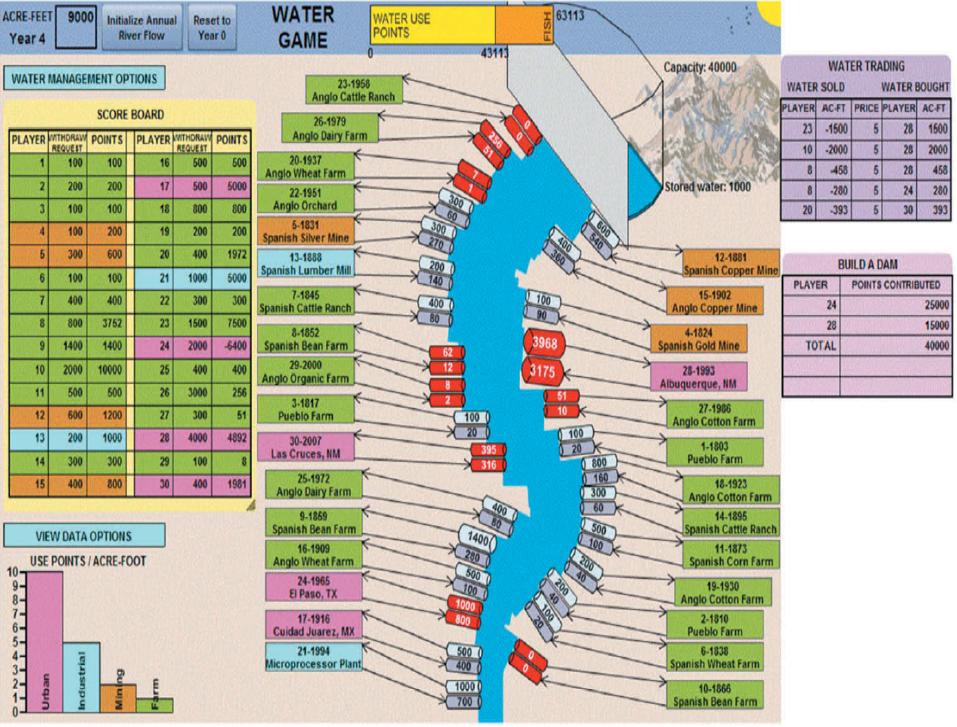
Players can address this unacceptable situation through three management options: (1) setting a minimum flow requirement for fish, (2) trading or leasing water among users at agreed-upon prices, and (3) building a dam to store water from wet years for subsequent dry years. While each player’s goal is to maximize their own water points, the overall goal is to maximize river-wide water use plus fish habitat points. The randomness of water flows, the many possibilities for trading, and the interaction among management options capture some of the essential complexities and dilemmas of allocating scarce water resources under the prior appropriation doctrine. The simulations is available at Weidong’s Projects Homepage. Enjoy!

The Mississippi Watershed and the Problem of Polluted Runoff

Climate change, Amazon deforestation, endangered charismatic species like polar bears, and natural disasters like major hurricanes and wildfires seem to get all the attention. Meanwhile, more subtle, but no less urgent, environmental problems like polluted runoff grind on right under our very nose. America’s signature river, the Mississippi, the fascination of Mark Twain and whose name kids use when counting seconds, is its greatest example. The Mississippi River has a problem of too little sediment and too much nitrogen.

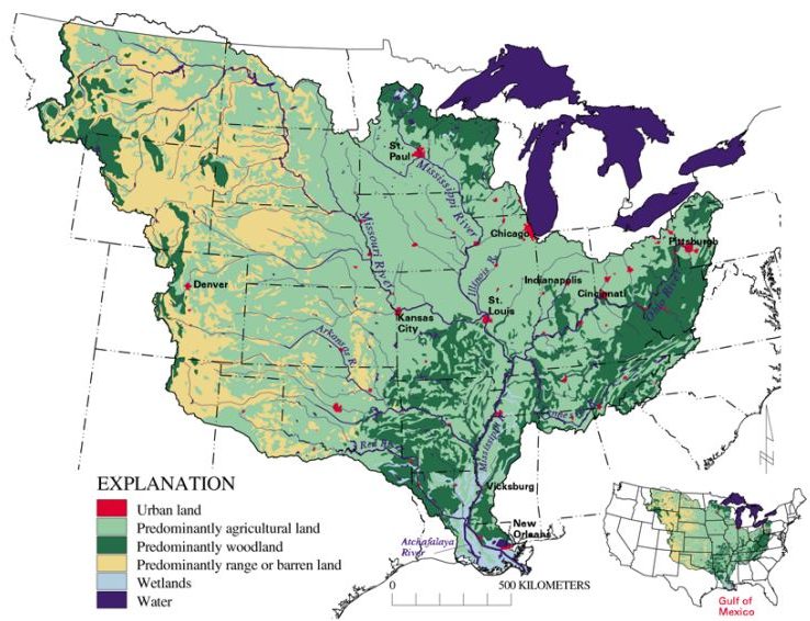
East to west, the Mississippi watershed stretches from the Appalachian crest from New York to Georgia to the continental divide from Montana to New Mexico. North to south it reaches from Alberta to its delta in Louisiana (Figure 12.9).

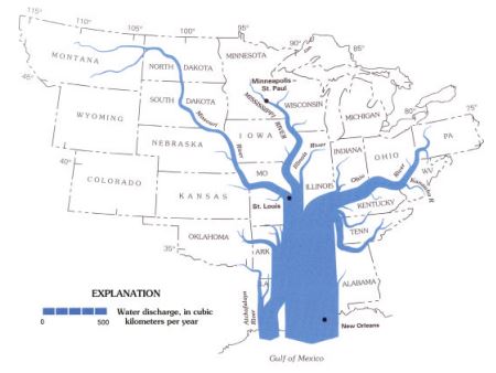
The basin contains America’s agricultural heartland as well as substantial areas of forest in the eastern portion and dry rangeland in the western portion. It has many cities, though on the whole is somewhat less densely populated than the U.S. average. Its largest tributary basin by land area is the Missouri, but its largest tributary river by volume of water is the Ohio. Its largest distributary (when they reach the delta, rivers usually divide into multiple channels) is the Atchafalaya (see water flow diagram in Figure 12.10), which would likely become the primary pathway to the sea, by-passing New Orleans, were it not for the Old River Control Structure preventing this with millions of tons of concrete.

The Mississippi and its major tributaries are barge superhighways carrying vast tonnages of coal, grain, timber, and other products from as far upstream as Sioux City, Iowa, on the Missouri, Minneapolis on the Upper Mississippi, and Pittsburgh (where the Allegheny and the Monongahela join to form the Ohio) to the port of New Orleans, and from there to the world and back again.

All rivers carry not only water but vast quantities of sediment to the ocean. This process slowly erodes away the land while nourishing the ocean and building a delta where the sediment drops out as the current wanes. The river system that Lewis and Clark traveled two centuries ago from Pittsburgh to the Continental Divide featured a clear Ohio, with its forested watershed holding the soil and filtering sediments. When they turned north and upstream, they encountered a muddy Middle Mississippi, though the turbidity disappeared as they gazed up the clear Upper Mississippi north of the Missouri River junction near St. Louis.

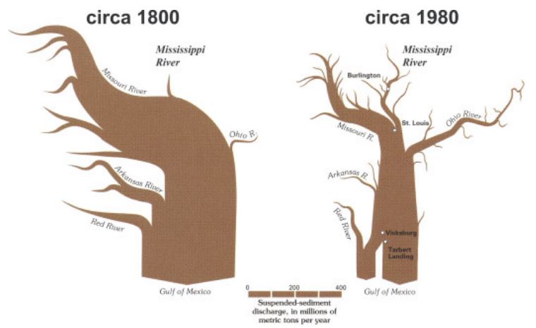
Getting started up the Missouri, they found a river too thin to plow and too thick to drink. Like the Yellow River in China, the Missouri carried an enormous sediment load borne from natural erosion on the glacial loess soils of Iowa and Nebraska and from the Great Plains—too dry to completely cover the land in a protective blanket of vegetation, yet regularly experiences intense erosive downpours. Other Great Plains tributaries like the Platte, Arkansas, and Red also contributed to the stupendous sediment load of 400 million tonnes per year (Figure 12.11). These sediments built most of Louisiana as the delta wetlands growing upon them stretched farther and farther into the Gulf of Mexico, protecting New Orleans from the storm surges of periodic hurricanes.

Human use of the river basin was to change the patterns of that sediment flux. Soil erosion resulting from agricultural development in the Ohio and Mississippi watersheds increased sediment loads from low to moderate. In the Missouri Basin, the Fork Peck, Garrison, Oahe, Big Bend, Fort Randall, and Gavins Point Dams were constructed by the Army Corps of Engineers between 1937 and 1963, ostensibly to provide water supply, control flooding, and improve navigation of the river by barges.

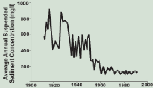
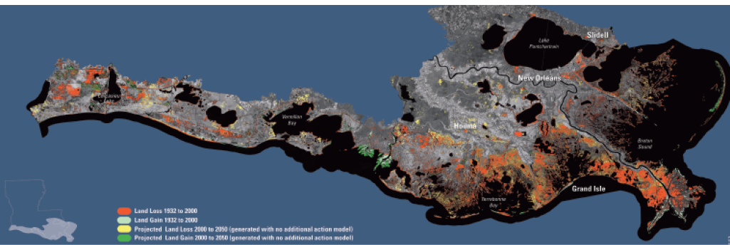
With the closures of the Garrison, Fort Randall, and Gavins Point dams in 1954 and 1955, the river’s enormous sediment loads immediately began to fill up these reservoirs with silt, while the river’s sediment load was reduced by at least three-fourths (Figure 12.12). The effects were felt locally as the hungry Missouri began to dig deeper into the loess and, in so doing, forcing all of its tributaries to do likewise, thereby producing a landscape of biologically impoverished entrenched streams undermining bridges across western Iowa and eastern Nebraska. The effects of reservoir sedimentation were also felt all the way to New Orleans as the river’s sediment load plunged. With the river contained within levees to facilitate navigation, what sediment remained was deposited 100 miles southeast of New Orleans, bypassing the delta almost altogether. With sea levels beginning to rise due to climate change, and oil and gas extraction accelerating natural subsidence, the sediment-starved delta began to sink and erode away—rapidly. It is estimated that since 1950 Louisiana has lost 1,900 square miles, an area about the size of Delaware (Figure 12.12). Moreover, this loss of protective wetlands has left New Orleans extraordinarily vulnerable to storm surge impacts of hurricanes as was tragically witnessed in 2005 with Hurricane Katrina.

In response, new ideas are being placed on the table. One is to build storm surge barriers east and south of New Orleans to block the sea from again invading the city. The first $1.1 billion phase of a $14.7 billion Army Corps of Engineers project is complete—a 2-mile-long seawall 10 miles east of New Orleans. Another idea works more closely with nature—redistribute the sediment to rebuild the delta. Even with its reduced sediment load, well-planned breaks in the levees containing the Mississippi to create new distributaries could accumulate lobes of silt, reversing the erosion process and creating new wetland environments. It would take decades, however, before New Orleans was again protected from hurricanes by a restored delta. Removing a Missouri River dam—especially the farthest downstream one at Gavins Point—to release more silt could also help. Restoring the Mississippi delta is an opportunity to practice adaptive management—learn by doing—while making its habitation more sustainable.

And then there’s the problem of too much nitrogen. As we’ve seen, nitrogen causes eutrophication by fertilizing algae, which consume oxygen when they die, creating hypoxic conditions. Oxygen-breathing creatures such as fish either die or move on. The Gulf hypoxic zone set a record area the size of Maryland in 2019, but the majority of streams and rivers feeding the Mississippi are also eutrophic, as is that great river itself.

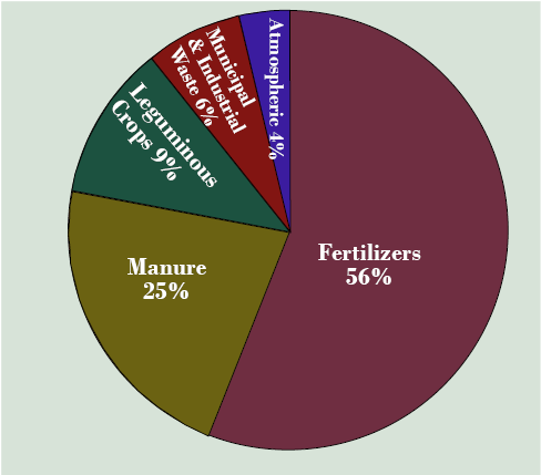
Where does all that nitrogen come from? The 2008 National Research Council study identifies fertilizers as the source of over half, followed by manure contributing one-fourth (Figure 12.14). Leguminous crops like soybeans are the third leading source. It’s mostly coming from Midwestern agriculture.

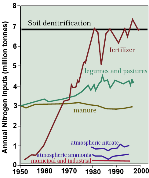
In 1950 manure, legumes, atmospheric, and industrial sources of nitrogen roughly balanced (at about 7 million tonnes per year) soil mineralization—the denitrification that anaerobic bacteria provide as an ecosystem service, mostly in wetlands. Since 1950, however, fertilizer runoff has climbed from almost nothing to about 7 million tonnes (Figure 12.15), doubling the input of nitrogen and overwhelming the denitrification process. The result is nitrogen overload and the undermining of aquatic and marine ecosystems.

Why is this happening? Just like the atmosphere can be overused as an open-access sink for carbon, the Mississippi watershed is being overused as an open-access sink for nitrogen. Farmers and feedlot managers do not pay a fee to use the watershed as the dump for their excess nitrogen, nor are there limits or caps on how much they can allow to run off. So, as in Hardin’s tragedy of the commons, this congestible resource is overused. Moreover, wetlands, as nature’s kidneys, encourage denitrification. Except through the Wetland Reserve Program mentioned in Chapter 11, no one gets paid to convert low-lying cropland to wetlands to provide this ecosystem service. So, in the tragedy of ecosystem services, it isn’t provided in sufficient quantity. In fact, over three-fourths of the wetlands in the Mississippi Basin have been drained, largely to expand agriculture.

Moreover, each state is responsible for the quality of water in their streams and rivers and submit lists of those requiring pollution reductions to the Environmental Protection Agency’s Total Maximum Daily Load (TMDL) program. Unfortunately, the Mississippi River forms state borders from Minnesota-Wisconsin to Louisiana-Mississippi, so it’s an orphan in the state-based TMDL process. Here we see again how a legal and institutional economic approach reveals a pattern of incentives that generates a problem rather than resolving it.

In the nitrogen simulation described in Chapter 3, you can utilize two potential solutions to Gulf hypoxia, fertilizer reductions and wetland restoration, to attempt to eliminate or minimize the hypoxic zone within a set budget. See how well you can do.

Two Global Water Issues Critical to Water Resources Sustainability

It is often stated that at least one billion people on Earth do not have access to safe drinking water through a treatment system such as we described above. About twice that number lack access to basic water sanitation—a septic or sewer system. Most Americans cannot imagine the human cost of this lack of water resources development. Over two million babies and young children die every year from diarrheal diseases from drinking contaminated water. Many other diseases of the poor, especially in the tropics, are water-related: cholera, typhoid, schistosomiasis, and guinea worm (a dreadful disease former President Carter’s Center is determined to eliminate). If these diseases could be prevented, infant and child mortality would plummet, and with it, the fertility rate (remember descendant insurance from Chapter 5). From there, economic development could gain a foothold, bringing the world’s poorest into a life of security and dignity. It has often been said that the best way to improve the world is to bring safe drinking water to those who don’t have it. It turns out that this is likely true.

There is a silver lining: it used to be worse. In 1970 only 30 percent of people in developing countries had access to safe drinking water and only 23 percent had working sanitation systems. By 2000, 53 percent had sanitation and fully 80 percent had access to treated drinking water. This represents one of the great untold success stories in sustainable resources management. The problem is never a lack of water; as we saw above, water for drinking and sanitation is a tiny fraction of water use. A mere 50 liters, about 12 gallons per person per day, can make the difference. Some have claimed that this should be a human right.

The problem is a lack of infrastructure along the lines shown in Figure 12.3, expensive water treatment and distribution infrastructure that nearly all Americans have enjoyed for about a century. Given the momentum generated over the past 50 years and the enormous benefits in controlling disease, it seems that delivering safe drinking water to nearly everyone is a goal that is both achievable and worthwhile. I put it first on the to-do list for sustainable water resources management.

Even if this goal is achieved, however, it still does not feed everyone. When green water is included, meat-rich and sometimes overabundant North America diets require about 1,200–1,300 gallons per day to produce. Largely vegetarian and sometimes inadequate African and Asian diets require about half as much. Where is this water going to come from in a world with an increasing population that is transitioning to diets that require much more water to produce? In much of tropical Africa, the problem is developing the water resources they do have for municipal supplies and irrigation. In the virtual water-importing regions stretching from North Africa, through the Middle East, South and Central Asia to North China, in contrast, the problem is lack of water resources to expand, or even maintain, irrigation.

In Pillar of Sand, Sandra Postel told how the Green Revolution, including the great expansion of irrigation, was the key to expanding food supplies to keep up with population growth in the populous continent of Asia over the past half-century. Like in the Colorado River Basin, however, in watershed after watershed, freshwater supplies have been fully developed. We examined the catastrophe of the Aral Sea in Chapter 2. The Yellow River of North China now sees intervals of months where not a drop of water flows to the Yellow Sea. The capital of Beijing is threatened with an inadequate water supply. China’s response has been a multi-billion-dollar plan to build canals transferring a substantial portion of the voluminous Yangtze River northward to the Yellow basin.

Groundwater tables are dropping in north China and western India. The sources of the Indus River in Indian Kashmir, lifeline of arid Pakistan, are a lightning rod of conflict between India and Pakistan. Management of the Brahmaputra-Ganges has generated conflict between India and Bangladesh, management of the Mekong among the nations of Southeast Asia. Climate change is worsening the situation by melting the massive glaciers of the high Himalayas and Tibet that serve as the summer supply for all of these rivers. The water situation is even more severe in the even drier Middle East where Turkey, Syria, and Iraq have struggled over the waters of the Euphrates. Jordan, Israel, and Palestine share the trickle of water known as the Jordan River and aquifers along it.

These are the most pressing issues in water resources sustainability, but, as we discussed with reference to the American Southwest, there are solutions in more crop for the drop, crops that drink fewer drops, virtual water, and water reallocation. As in the dilemma of prior appropriation in the Western U.S., there are social, political, and economic barriers unique to each country and watershed to feeding more people with less water. The key is to diagnose what these barriers are and to overcome them. Who would have thought in 1970 that 30 years later 80 percent of people in developing countries would have access to safe drinking water? Who would have thought in 1980 that by 2020 total U.S. water withdrawals would have declined? Resignation is the enemy of the solution. Patient persistence is its friend.

The Ecological-Economic Value of Water

Fresh water has so many uses. Managing it consists of evaluating those uses relative to the resources available, in terms of both quantity and quality, over time and across space. The idea from neoclassical economics that scarce resources should be allocated to their highest and best use is sound, but in making that determination we need to work our way through market failures that provide the wrong incentives to managers and users. We also need to fully incorporate ecosystem services into the equation. The market value of water to users—usually as a factor of production of crops, energy, or a clean and healthy home, business of facility—represents what they are willing to pay for it. There are two more critical values of water, however, that escape neoclassical economic analysis. The first 50 liters of safe drinking water per capita per day, the water lifeline, is essential to public health and thus saves lives, especially babies and small children. It thus has a huge value to people, preserving human capital, whether it generates an “economic” value or not. Finally, water in its natural settings, in lakes, streams, wetlands, and so forth, is, as we have seen, the most critical factor of production of ecosystem services. In fact, ecosystems defined by fresh or shallow salt water (e.g., estuaries, wetlands, aquatic) have the greatest ecosystem service value per unit area.

What is the opportunity cost of using water for one purpose rather than another? The costs of supplying water that a user must pay for include the cost of building the water supply system we described above, plus operation and maintenance of that system. That excludes any charge for the water itself, however, especially the value of the alterative use that could have been made of it. It also excludes economic externalities such as the degradation in the quality of the water that inhibits other uses. It is in this sense that neoclassical economists have argued that water is underpriced—all the costs for using it are not paid for by the user. In ecological economics, this argument goes even further because when water is consumed or degraded in quality, the ecosystem services that water could have generated are lost. Except in conditions of flood, there is, at the margin, an ecological-economic opportunity cost. Water used to irrigate crops is water no longer available for salmon spawning, as in the case of the Klamath River, or the survival of an endangered fish species, as in the case of the Rio Grande, or for denitrification and bird habitat in wetlands, as in the case of the desiccated Colorado River Delta.

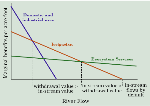
Figure 12.16 analyzes these trade-offs for a hypothetic western river. The marginal benefits, the ecological-economic value of one more acre-foot, is shown on the y-axis. On the x-axis is the flow of the river from the first trickle on the left to bank-full flow on the right. The value of domestic and industrial uses is high, but these diminish quickly as needs are met. Irrigation values are not as high, but they diminish more slowly as land less and less suitable for irrigated agriculture and less and less valuable crops are brought into production. For the first acre-foot of water, ecosystem service values are probably not quite as high, but every acre-foot counts, expanding the services that can be delivered from streams, wetlands, and riparian zones.

Highest and best use represents the highest value use at each level of river flow. For the first increment of river flow, this is domestic and industrial uses that keep people healthy and generate large numbers of jobs. Once these needs are met, additional river flow can be allocated to either irrigation or left in the natural watercourse for ecosystem services. If the value of the latter is excluded, farmers will use water until its marginal value is zero, leaving limited in-stream flows only when they can’t earn additional income from the remaining water. But water left in the stream or reservoir for ecosystem services can exceed values for irrigation. A point is reached where the highest and best use is in-stream flows. In fact, when the long-term viability of a species or salmon run is at stake, the value of an acre-foot in the stream may exceed any possible value in irrigation. When ecosystem service values are not considered, too much water is withdrawn from the stream and the highest and best use of scarce water is not realized. This is unsustainable as well as inefficient. Virtual water can play an important role here by trading food from water-abundant regions, where irrigation and ecosystem services are not in competition for scarce water, to water-deficit regions so that the latter can maintain in-stream flows, aquatic ecosystems, and their biodiversity and services.

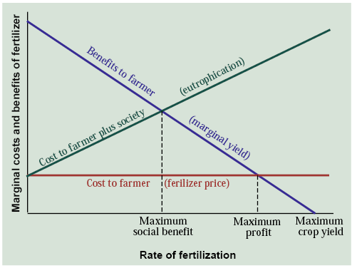
A similar logic applies to water quality, again especially in an agricultural context. Take the nitrogen overload problem in the Mississippi discussed above, which results from heavy rates of fertilization. In Figure 12.17, the marginal costs and benefits of adding more fertilizer to crops are shown on the y-axis and the amount of fertilizer applied along the x-axis. Starting from zero, as fertilizer is added, crop yields, and thus revenue to the farmer, increase, but at a decreasing rate due to diminishing marginal returns. At some point (where the benefits to farmer line crosses the x-axis), crops stop responding to more fertilizer. Farmers wishing to maximize their crop yields would stop adding more fertilizer at this point. Fertilizer must be paid for, however, and its price represents the marginal costs to farmers of adding more. To maximize profits rather than yield, farmers would stop adding fertilizer at the point where the revenues from additional yields fall below the cost of the additional fertilizer.

At this point farmers are still overfertilizing because there is also a social cost to fertilization that comes in the form of eutrophication and the associated loss of ecosystem values. These costs climb as more and more fertilizer is added, overloading the watershed with nitrogen. When this is figured in, the time to stop adding more fertilizer is shown where the marginal cost and benefit curves cross and social benefit is maximized. This lower level of fertilization represents the best balance between food production and protection of aquatic and marine ecosystems. If it were widely employed, the Mississippi River story told above would be a much more sustainable one, and you and I may never have heard of Gulf hypoxia.

From National Water Resources Development to Local Integrated Water Resources Management

Over the years, I have heard frequent calls for a national water policy or to restore the defunct National Water Council. I’m unconvinced. As Massachusetts member of the House of Representatives Tip O’Neil once said of politics, all water issues are local. States own the water within their boundaries. Except for a few communities that have taken the privatization route, local governments provide drinking water and wastewater services for their citizens. Moreover, the nature of water resources management problems is changing in a way that makes localities the playing field even more than in the past.

As told by Marc Reisner in Cadillac Desert, for most of the 20th century U.S. water issues focused on water resources development—capturing freshwater, usually with a dam, before it escapes to the sea and bringing it to bear as a factor of production for growing cities, industry, power production, navigation, and agriculture. Dams and levees were constructed to try to contain floods. It was the territory of the civil engineer working for a federal agency such as the Army Corps of Engineers or the Bureau of Reclamation and of members of Congress bringing home the bacon in the form of a federally funded water project.

After the Clean Water Act passed in 1972, the focus shifted to environmental infrastructure, especially the construction of wastewater treatment plants. Civil engineers became environmental engineers, and Congressmen brought home earmarks rather than barrels of pork. In their own fashion, developing countries like Brazil, China, and India are still working through this era of water resources development, and tropical Africa has begun it.

We are now two decades deep into the 21st century and the playing field has changed remarkably. The great era of dam, levee, and drinking and wastewater treatment plant construction is over. Those infrastructures are in place, even if many, especially in the older eastern cities, have suffered from deferred maintenance. The issues of this century revolve around sustainability and working locally with nature to meet human needs. These include irrigation efficiency and institutional mechanisms to reallocate water from low-value uses to other purposes, managing urban water demands, and controlling urbanization of floodplains. Controlling polluted runoff and restoring wetland and aquatic ecosystems that water resources and land development has left in a degraded state are even more locally oriented issues.

The federal agencies of the 20th century—the Army Corps of Engineers and the Bureau of Reclamation—can be helpful here but as occasional consultants and contractors hired by locally-controlled initiatives. Rather than the primary funder of engineering projects, the new, more limited role of the federal government is primarily to gather and disseminate data, to conduct research with shared results, and to provide the right incentives for conservation.

Instead, we need stronger local watershed-based institutions, perhaps resembling school, fire, and other local service districts. In order to be effective, watershed service districts need four characteristics. First, integrated watershed management should promote a shift from single-purpose management (e.g., water supply, flood control, wastewater treatment, stormwater control) to managing the watershed as a human ecosystem, where each of these elements interact. Second, the districts may require powers other forms of local government possess such as the authority to enact regulations, create economic incentives, administer permits, and conduct public information campaigns. They would also need to be funded through traditional means such as taxes, fees, and bonds. Third, they need the institutional capacity (e.g., budget, staff, and expertise) to manage a critical natural resource sustainably. This includes carrying out complex scientific and economic analyses and managing regulatory and permit programs. Fourth, they must be perceived as legitimate by the local community by holding elections for officers who conduct the public’s business in a transparent manner and are held accountable by the public for decisions made.

Summary

Freshwater is a subtle resource because we use it in many ways that slip beneath the radar screen of our popular culture. It is the key component of functioning ecosystems, yet these ends are often subordinated to the needs of energy, agriculture, urban development, navigation, and public health. Fortunately, as long as the hydrologic cycle keeps bringing rain and snow, we have the opportunity to make water resources management more sustainable by managing human needs within the context of watersheds as human ecosystems. Water teaches us that sustainability is more than just leaving some resources in the bucket for the next generation. It is also about keeping ecosystems—for which water is like blood for our bodies—functioning so that they may serve us in perpetuity.

Further Reading

Chapagain, A.K. and A.Y. Hoekstra, 2004. Water Footprint of Nations: Volume 1: Main Report. UNESCO-IHP Institute for Water Education.

Reisner, M., 1993. Cadillac Desert: The American West and its disappearing water. Penguin Books.

Solomon, S. 2010. Water: The epic struggle for wealth, power, and civilization. Harper Collins.