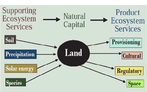
From a natural resource and ecological perspective, land is a package of supporting ecosystem services such as physical space, the soil covering it (if there is any), a place for precipitation and solar energy to interface with the soil, and the species of plants, animals, and microorganisms that inhabit that space (Figure 11.1). Collectively, these form natural capital in the sense we discussed that concept in Chapter 7 on ecological economics. As a unit of natural capital, land is capable of producing provisioning, cultural, and regulatory ecosystem services. Not all lands were created equal, however. The cold, nearly soilless northern Canadian Shield or the desert basins of Utah and Nevada, for example, have far less value as natural capital than the prime farmlands surrounding the Chicago metropolitan area or the scenic seacoasts of California’s climatic paradise. We obviously need to identify the factors that make land more or less valuable as a natural resource.

Three of these factors are the mantra of real estate traders: location, location, location. For example, commercial establishments prefer high traffic areas in attractive parts of town or interstate exits. For industries, adjacency to transportation facilities and proximity to raw materials and markets are key geographic factors. For homes, proximity to schools, churches, restaurants, shopping, and other nice homes is key along with a lack of pollution, crime, and visual blights like warehouses, rail yards, and interstate highways. We will not dwell here, however, on these geographic factors of urban land development where the primary service land provides is developable space. Instead, our focus will be on the agricultural and ecological value of rural lands, over 95 percent of all lands on Earth as well as in the U.S., as units of natural capital. Are these lands being managed in a manner that sustains their capacity to produce ecosystem services for human welfare, including the majority of humanity that lives in towns and cities? If not, what needs to change?

The Acquisition and Disposition of Land in the U.S.

The United States of America is a large country and this did not happen by accident; the 84 years from 1783 to 1867 witnessed a national territorial expansion equal to any other in world history. From thirteen British colonies hugging the Atlantic, the Treaty of Paris with Britain in 1783 established the new country’s boundaries from the Great Lakes and St. Lawrence River in the north to then-Spanish Florida in the south, west to the Mississippi River (Figure 11.2). Yet, west of the Alleghenies (a prominent ridge in the Appalachian chain), the land was “Indian Country” being steadily encroached upon by settlers. Only 20 years later in 1803, Ambassador Robert Livinstone reported to President Jefferson that Napoleon of France, indebted by war and withdrawing from American colonial ambitions, was interested in selling all of France’s North America lands west of the Mississippi, not just the mouth of the Mississippi in Louisiana. Despite constitutional reservations, the U.S. took the sweet deal. Then in 1818 the U.S. compromised with Britain on the 49th parallel, rather than the divide demarcating the Mississippi watershed, and in 1819 leveraged Florida from Spain.

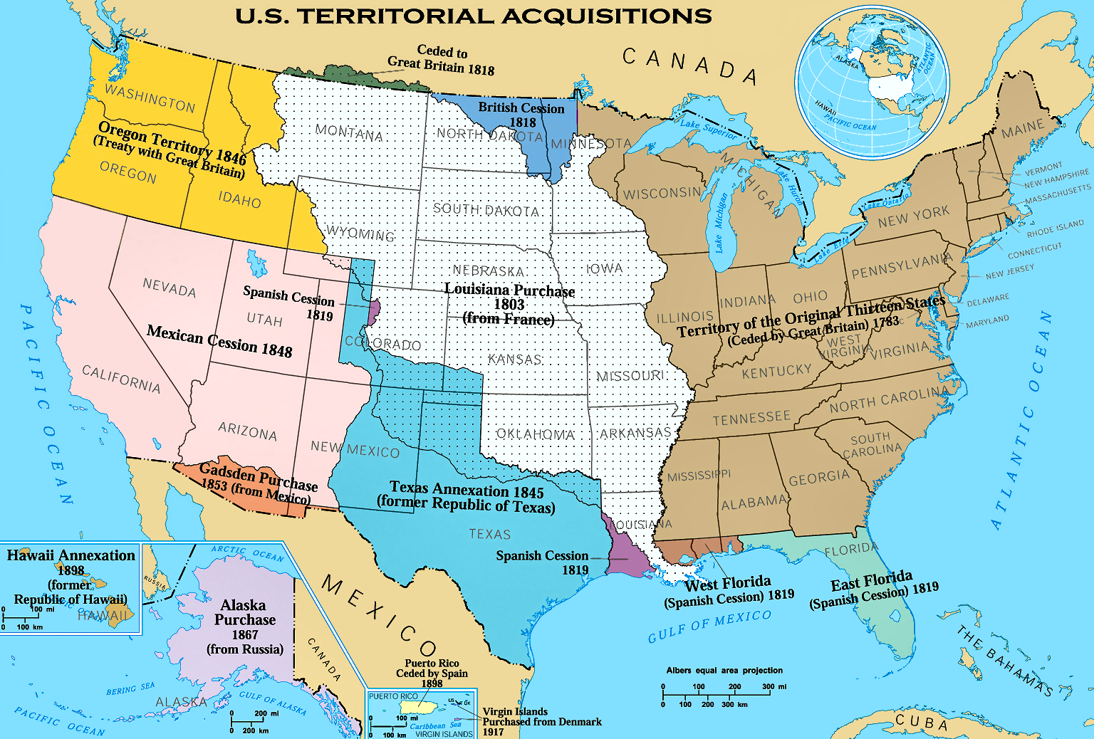
The next round of territorial acquisition came in the 1840s when the U.S. observed that newly-independent Mexico’s hold on its northern lands was tenuous. Annexation of the briefly independent Republic of Texas and the Mexican session followed a short brutal war initiated by the U.S. imperialist claim to “manifest destiny.” Another war with Britain was avoided by the Oregon Compromise of 1846 that extended the northern border along the 49th parallel to the Pacific. Finally, the U.S. purchased Alaska on the cheap from Tsarist Russia in 1867. Some territorial changes have occurred since 1867 but all Americans living today have enjoyed these stable national borders.

Whether annexed, purchased or otherwise acquired from European and North American powers, all of these lands were wrested from indigenous peoples, usually following a similar process. Treaties were negotiated between the U.S. government and the various Indian tribes guaranteeing protection of native lands. Settlers ignored them and encroached on whatever lands they wanted and thought they could defend from Indian counter-attack. Democratically elected governments refused to enforce the treaties they had signed, bending to popular pressure, making these encroachments an on-the-ground fact. Indian peoples moved west or became marginalized.

In perhaps the most tragic episode of all, in 1830 President Jackson signed the “Indian Removal Act” forcing the Creek, Cherokee, Chickasaw and other indigenous peoples to march along the “Trail of Tears” from their historic homelands in the southeast to their “permanent” new home in Oklahoma. Yet on April 22, 1889, 50,000 “sooners” rushed in to claim these native lands. The march west continued through the end of the 19th Century by which time the few hundred Indian Reservations occupying 2.3 percent of U.S. area had been established.

With the exception of the Republic of Texas, in each of these episodes of territorial acquisition, native lands fell into the hands of the U.S. government with Congress busily debating what to do with them. and the courts attempting to resolve an onslaught of disputes Securing these newly acquired lands permanently and developing the country required encouraging pioneers to settle the western frontier and, when the time came, to admit new states into the union on an equal basis with the original states. By 1912 the 48 conterminous states had been admitted to the union: Alaska and Hawaii were added in 1959.

Throughout the 19th century, the U.S. government was focused on “disposing” the recently acquired lands to private individuals and companies who would form the new states. The process was chaotic and rife with corruption, yet it was also rapid and effective, with the frontier “closing” in the 1890s. Policies governing mineral, wildlife, timber, water and other resources encouraged a race to the west to be the first to lay claim to these resources that lay within the new lands that had been precisely laid out into square mile sections and townships. The Homestead Act rapidly established a farming-oriented white population throughout the ecologically productive and fertile Midwest but, west of the 100th meridian, which runs through the center of the 48 states, aridity made 160-acre rainfed homesteader farms unviable due to lower ecological productivity.

John Wesley Powell, the daring explorer of the Colorado River and father of the U.S. Geological Survey, argued that Midwestern-style homesteads would not work in the arid and mountainous West. Rather, with a few exceptions such as the fertile Williamette Valley of Oregon, destination of the Oregon Trail, a viable farm needed perhaps 40 acres of communally organized, highly productive irrigated cropland joined, except in the Central Valley of California, to several square miles of ecologically unproductive rangeland. Since water was the limiting factor in human development in the West, states should be organized on the basis of river basins. Had Congress taken Powell’s advice, western states would be named “Columbia,” “Snake,” “Sacramento,” “North Colorado,” South Colorado,” “Rio Grande,” and “Great Basin.” The stories of the wild west, rife with lawlessness and conflict borne of desperation, would have been much tamer.

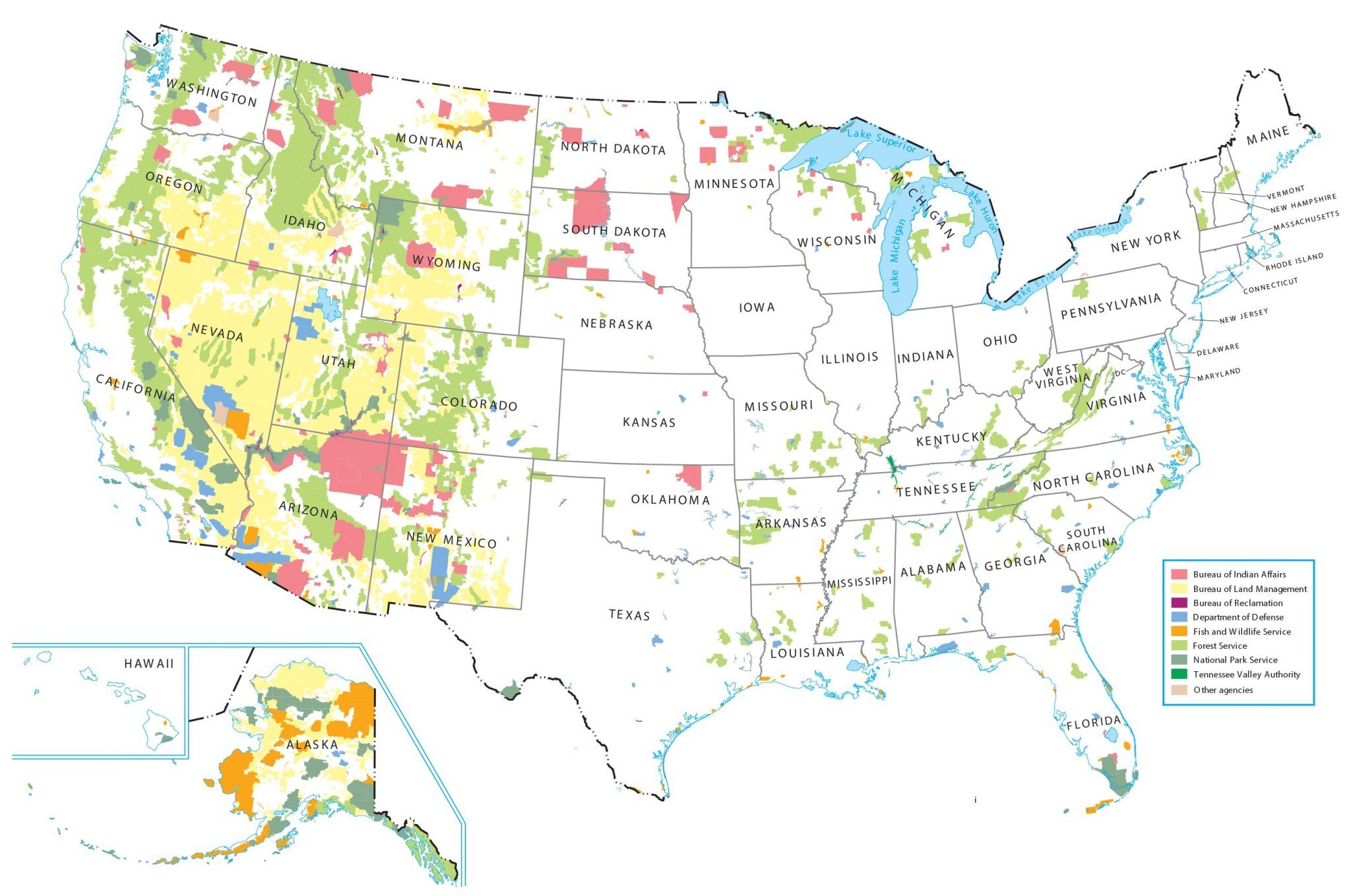
While the scattered agriculturally viable lands of the West were “disposed” as they were east of the Rocky Mountains, most lands could not be settled with substantial rural populations and the majority therefore remained in federal hands. Today, Federal Lands occupy 28 percent of the U.S., divided among the Bureau of Land Management (BLM), National Parks and Fish and Wildlife Refuges (all in the Department of Interior), and National Forests in the Department of Agriculture (Figure 11.3). Yet these percentages vary from 80 percent in Nevada, 46 percent in the 11 western states as a whole and 61 percent in Alaska. In contrast, federal lands are no more than 14 percent of any state east of the Rockies and less then 2 percent in 13 eastern states.

In 1872 Yellowstone became the first of 63 National Parks, the gems of the federal land system managed by the National Park Service for preservation balanced with managing ever-multiplying visitors that reached a record 300 million in 2021. First established in 1891 to protect mountain watersheds from excessive deforestation and erosion, the 154 National Forests are managed for recreation alongside grazing and timber supply, among other uses prescribed in the Multiple-Use Sustained-Yield Act of 1960. The first of 550 National Wildlife Refuges was established in 1903; they are not concentrated in the west and span every habitat type but emphasize wetlands with their high biodiversity.

While the largest in area, Bureau of Land Management lands are ‘leftovers’ from the original federal domain that aren’t suitable as national parks, forests, or wildlife refuges and were not claimed by 19th Century settlers. On these vast semi-arid to arid lands, including two-thirds of Nevada, the BLM balances often-competing recreational uses with natural resource extraction, from sparse grazing to intensive mining and, more recently, renewable energy development.

Our concept of property, and the evolution of that essential legal idea, is based fundamentally on land. Urban development and agricultural production occur overwhelmingly on private land where investments sown create the right to reap. Yet much of what happens on land affects neighbors, communities, ecosystems, watersheds, even the planet, in ways that are essentially public. How the U.S. came to acquire and then divide its lands into private and public spheres is thus a building block of a deeper understanding of land as a resource.

Land Cover and Land Use

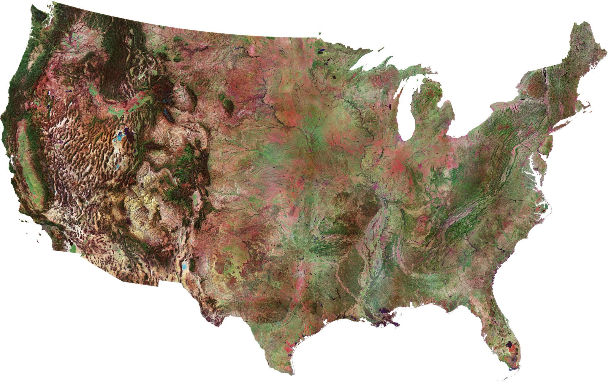
Figure 11.4 shows what a satellite sees when it looks at the contiguous 48 U.S. states. The interesting technical field of remote sensing is the art and science of rigorously analyzing the raw data that generate a satellite image to determine what is actually on the ground, often to place it into a category of land cover. It can be a challenge to, say, determine which field has corn and which has soybeans, which grassy place is a cattle pasture and which is a backyard. Remote sensing images can also be used to detect changes in land cover due to urbanization, deforestation or reforestation, changes in agriculture or climate.

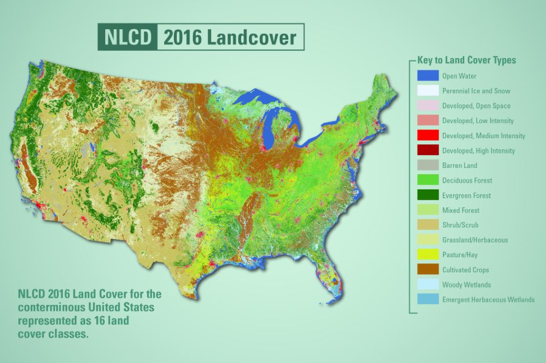
Using satellite image analysis methods, a land cover map of the U.S. was generated by the U.S. Geological Survey, as shown in Figure 11.5. Note how vegetation, the first trophic level and foundation of ecosystems, is the primary criterion for classifying land cover. Figure 11.6 adds up the land uses in each of eight categories in the form of a pie chart. Note that the development of these categories involves judgment calls, for example, how many different categories of forest should there be? Even after the categories have been decided, how many trees does it take to turn a grassland into a forest? Are the lily pads along the fringe of the lake freshwater or wetlands? More critically, is the landscape really divided into clearly urban and clearly rural locations? These questions have to be decided by reasonable rules of thumb but they always entails over-simplifications that can distort our understanding of the real world they portray. Data on land use change, such as rates of urbanization or tropical deforestation, are based on these agreed-upon rules as to what constitutes land in one or another category in a world that, on the ground, contains every shade of ambiguous gray.

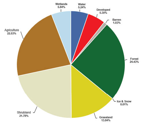
Having provided these caveats and clarifications, you may be surprised to find that one of the largest categories of land cover in the contiguous U.S. is shrub/scrub at 22 percent. This represents the large areas of the western U.S that are semiarid sagebrush and arid cactus country. Cultivated crops cover 16 percent, especially in the Midwest; together with pastures, agriculture occupies a critical 22.5 percent of U.S. land. Grasslands, dominant in the Great Plains, occupying 14 percent. About a quarter is forest, with mostly evergreen or coniferous common in the western mountains and the sandy southeastern coastal plains while rural areas of the eastern U.S. that are too hilly or infertile for crops are mostly deciduous forest.

Developed land is about 5 percent but 3 percent of this is open space—backyards, parks, and grassy areas intermixed with 1.5 percent of low-density development; we call it the suburbs. Medium density, the city, is 0.7 percent, and only 0.25 percent is high intensity development that you would find on Manhattan Island in New York, the Chicago Loop, or other big city downtown areas.

Land use is conceptually different from land cover. It’s not just the vegetation, rooftops, or other things we see from above but the purpose to which the land is being put. By far the most prevalent land use is agriculture, occupying about half of all land when grazing and crops are summed, both globally and in the U.S. Agriculture in its many forms is therefore front and center in a discussion of land as a natural resource and is a central focus of this chapter. Forests also occupy one-fourth of the land surface, so forestry is our secondary focus. Agricultural and forest lands each generate both provisioning ecosystem services—food, fiber, and fuel—as well as cultural and regulatory ecosystem services. The mix among these, and the maintenance of natural capital so that ecosystem services can be provided in perpetuity, are the central issues in using land sustainably.

Forms of Agricultural Land Use

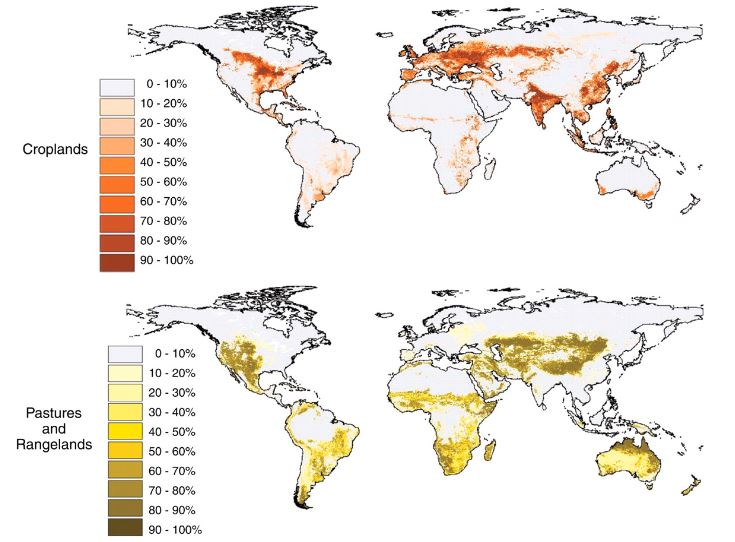
We’ve had several rendezvous with agriculture already, especially in Chapter 2 on Lessons from Environmental History. Agriculture is the deliberate manipulation of ecosystems to produce goods and provisioning services for humans, especially food but also fiber (e.g., cotton, flax, wool, wood) and fuel (e.g., wood, biofuels). Not coincidentally, the geographic distribution of cultivated areas (Figure 11.6 top map) matches well, but not perfectly, with the distribution of people on Earth. With some exceptions, land that can support agriculture defines the human habitat on Earth. Pastures and rangelands used for livestock (Figure 11.7 bottom) tend to lie in less densely populated regions that are not suitable for crop production due to aridity or soil infertility, yet they occupy even more land in total.

There are many forms of agricultural production. Here we simply need to identify some of the most important. First, we must describe two dichotomies. Commercial agriculture focuses on sale of commodities in markets. Subsistence agriculture produces food for local consumption. Intensive agriculture applies considerable labor and capital to achieve high yields per acre on highly fertile land. Extensive agriculture applies large areas of less fertile land to achieve more modest outputs per acre. With these dichotomies in mind, let’s briefly run down the legend in Figure 11.8.

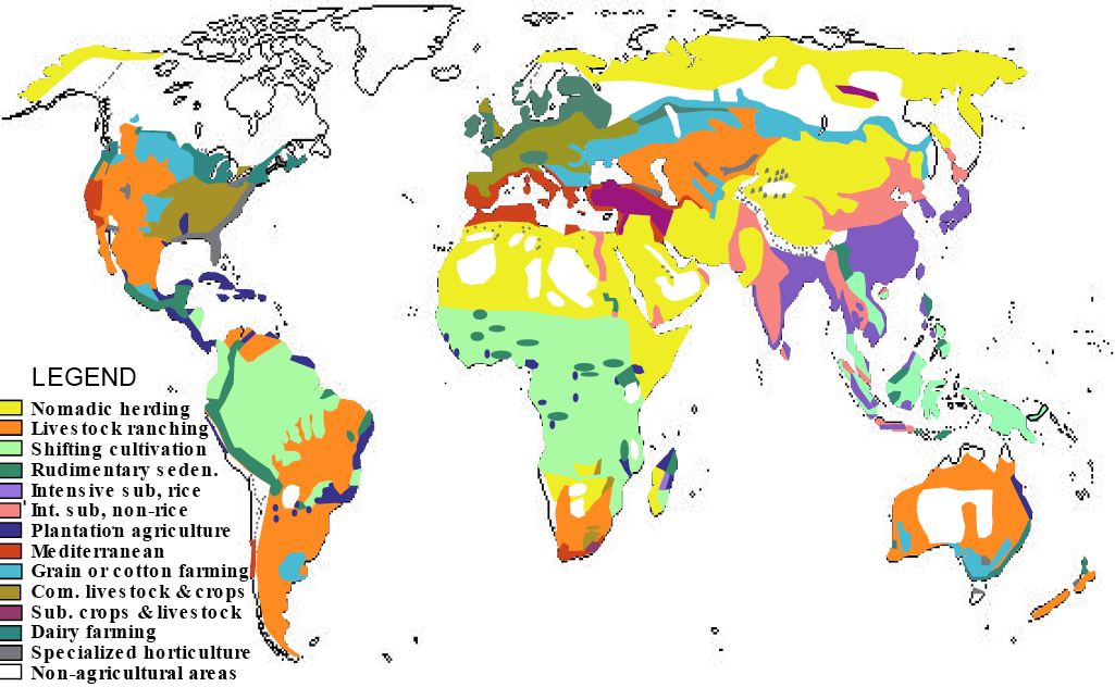
Nomadic herding occurs in arid and semiarid areas where sheep, goats, cattle, camels, or, in the sub-arctic, reindeer are moved frequently in search of greener pastures. It is an ancient but shrinking subsistence-oriented way of life in the Middle East and North Africa, Central Asia, Mongolia, and Siberia.

Livestock ranching occurs in similar environments, but on privately owned ranches, providing goods for commercial markets. It is common in drier grassland and shrubland areas of the western U.S., Latin America, Australia, and Kazakhstan.

Shifting cultivation uses the infertile soils but warm climates of wet tropical regions by periodically burning vegetation to release its nutrients into the soil as ash. It is extensive, usually subsistence in orientation, and seminomadic as farmers must move to new fields every few years as soil fertility declines. It releases enormous quantities of carbon and other pollutants to the atmosphere through forest burning. Shifting cultivation can be sustainable in tropical forests if population densities are low and fallow periods are long but it is becoming less and less viable as population pressure forces farmers to adopt more intensive approaches.

Rudimentary sedentary agriculture can replace shifting cultivation to meet food needs in developing countries in areas where soils will support permanent cultivation.

Intensive subsistence tillage employs hundreds of millions and feeds billions in the populous regions of South and East Asia. Rice, a very productive subtropical grain native to marshes, is dominant where growing seasons are long and water is abundant for flooding the paddies, such as in southeastern China, eastern India and Bangladesh, southeast Asia, the Indonesian island of Java, and the few flat valleys of southern Japan. Drier or cooler areas of Asia, such as western and northern India and northeastern China, often focus on wheat production in combination with a multitude of vegetable crops.

Plantation agriculture often focuses on tropical crops such as coffee, tea, cocoa, and bananas for export to temperate countries. Mediterranean crops such as grapes, olives, and avocados utilize the wet winters and dry summers of that region as well as of California.

Crop farming, in its commercial form, is common in subhumid temperate regions such as the wheat belts of the North American Great Plains, along the Russia-Kazakhstan border, the Pampas of Argentina, and southeast Australia.

Commercial livestock is the focus of crop farming in areas that have sufficient rainfall and soil fertility to support corn (called “maize” outside North America), often planted in rotation with soybeans. Most of the crop harvest is fed to cattle, pigs, and chickens with meat as the primary product, though increasingly corn is used for biofuels. This form of farming is very familiar to inhabitants of the Midwestern Corn Belt centered on Illinois and Iowa, as well as in Europe from France through Germany to Poland.

Dairy farming, where female cattle are fed from pastures, hay, and “silage” corn that has too short of a growing season to mature into grain, occurs to the north of commercial livestock areas both in Europe (the British Isles and Scandinavia) and North America (the Northeastern and upper Great Lakes states and southeastern Canada).

Specialized horticulture, common along the U.S. Atlantic coast and in parts of California, focuses mainly on fruit orchards and vegetables, often on small, productive farms near urban markets for fresh produce. It is a small percentage of agricultural land, but it produces some of the highest quality food products.

The Challenge of Agricultural Sustainability

A 2011 paper on “Solutions for a Cultivated Planet” in the prestigious journal Nature summarizes the challenge of agricultural sustainability well:

Increasing population and consumption are placing unprecedented demands on agriculture and natural resources. Today, approximately a billion people are chronically malnourished while our agricultural systems are concurrently degrading land, water, biodiversity and climate on a global scale. To meet the world’s future food security and sustainability needs, food production must grow substantially while, at the same time, agriculture’s environmental footprint must shrink dramatically.

Increase food production and decrease the resources used to produce food at the same time? This seems like quite a trick to pull off! Yet there are reasons to think it is quite possible by following some straightforward strategies as we will see below.

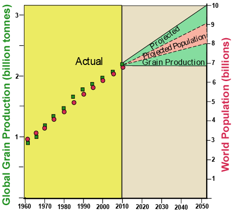
First, let’s look at the food-population balance and how it has been evolving. Population was rapidly increasing, doubling from about 3 to 6 billion in the period 1960–2000 but has slowed in the 21st century, as we explored in Chapter 5, to reach 8 billion in 2022. Has global food production kept pace? If we focus on grains (rice, wheat, and corn provide 60 percent of human calories), we can see from Figure 11.9 that it slightly more than doubled from 0.9 to 2.2 billion tonnes from 1960–2010 and was 2.3 billion tonnes in 2021.

How was this enormous increase in grain production achieved? Did the area in crops expand? It turns out that cropland area since 1960 has been very stable in Eurasia and North America though it has expanded in Africa and South America. Eastern South America in particular represents the planet’s agricultural margin, reflecting the overall supply-demand balance. Even during the most rapid increase in human population in history, only in Brazil has substantial new cropland been brought into production. This tells us that the world’s farmers have already found the fertile and resilient lands and few remain open for agricultural expansion. What does remain is primarily tropical forest, a great storehouse of biodiversity and carbon that many would wish to conserve.

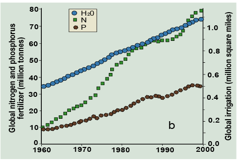
Fortunately, yields on cropland doubled from 1960–2000 as shown in Figure 11.10a. How was this achieved? Iowan Norman Borlaug is often called the father of the Green Revolution. He witnessed how the use of higher-yield varieties of grain and the application of chemical fertilizers, especially nitrogen, and irrigation water in drier regions could greatly increase crop yields. He made it his life mission to bring these benefits to developing countries in order to combat world hunger and won the Nobel Peace Prize for these efforts. Figure 11.10b shows how an 8-fold increase from 10 to 80 million tonnes in nitrogen fertilizer, a tripling in phosphorus application from 10 to 30 million tonnes, and a doubling in area irrigated from 0.14 to 0.28 billion hectares (540,000 to 1,080,000 square miles) resulted in a doubling of grain yields from about 14,000 to 28,000 hectogram per hectare (3.8 to 7.6 tons per acre). The doubling of crop production that occurred from 1960 to 2000 was due 71 percent to increases in yields and only 21 percent from expansion of area cropped. The remaining 6 percent was due to more double-cropping. It seems as though Borlaug’s formula has worked.

Unfortunately, it’s not that simple. First of all, political ecologists and others have argued that it is primarily the larger commercial farmers that have achieved the higher yields because they are the ones who can afford the fertilizers, irrigation developments and cutting-edge seeds. Smaller subsistence farmers have often lost their market and ultimately their land in the process. So even if there is more food produced, there are also more desperately poor people in rural areas who can’t afford to buy it. Often these hungry economic refugees end up swelling the slums and shantytowns surrounding many cities in periphery countries.

There is also an ecological critique. As we explored in the context of ecological limiting factors, crops can only absorb so much fertilizer and water. In 1960 every pound of nitrogen fertilizer applied yielded 80 additional pounds of grain. By 1980 this had fallen to 20 pounds, where it has remained. Once adequate nitrogen and phosphorus fertilizer has been applied, adding more fertilizer does not increase crop yields appreciably. In fact, less than half of global fertilizer applications are taken up by crops. The rest pollutes water as we explored in Chapter 3. Irrigation water increases yields only to a point as well and, as we will explore in the next chapter, many areas are running very short of fresh water. These watersheds and aquifers may not be able to maintain the quantities now used for irrigation, no less expand them. So, Borlaug’s Green Revolution seems to have largely played itself out. Except in sub-Saharan Africa, we cannot expect additional inputs of fertilizer and irrigation water to increase crop production at anywhere near the rate achieved over the past half-century. Worse, fertilizers have become the most widespread source of water pollution on Earth, and nitrogen fertilizers can evaporate to form nitrous oxide, a powerful greenhouse gas and a contributor to acid rain. Moreover, irrigation places far more strains on freshwater resources than any other use. Rice paddy agriculture and livestock are the leading sources of atmospheric emissions of methane, the second leading greenhouse gas.

There are other constraints to increasing agricultural yields as well. The health of crops can often only be maintained through an ongoing technological race against the biological process of natural selection. New hybrids of corn, rice, and wheat must be developed every few years to maintain resistance against fungal and other diseases. Weeds develop resistance to herbicides in a decade or two. More antibiotics are fed to livestock than to humans, yet resistant strains of bacteria usually develop in one to three years. This threatens the ability of antibiotics to control bacterial infections in humans as well, an enormous public health issue. Increasing agricultural production emerges as a natural resources sustainability dilemma of enormous proportions.

It gets even more challenging when we more fully consider pesticides, an umbrella term that includes herbicides (weed killers), insecticides, and fungicides. As Rachel Carson pointed out in her 1962 classic Silent Spring, many pesticides are persistent, meaning that normal ecological processes do not quickly break down these chemicals into ordinary harmless forms; they are not biodegradable. Worse, many also bioaccumulate; they become more and more concentrated as they move up the food chain. This tends to occur with chemicals that are fat-soluble because most of the fat that occurs in nature is in animal’s bodies, such as polar bears and humans. While some good work has been done to reduce pesticide’s risk to human health, their use remains widespread. Pesticides pose health risks in the form of cancer, neurological problems, and endocrine disruption, including birth defects, retarded brain development in children, and reproductive problems. In fact, sperm counts in human males have been substantially reduced worldwide. Pesticide exposure may play a role.

Climate change is now clearly slowly the rate at which crop yields are increasing. Heat waves are as devastating to most crops as they are to isolated elderly people lacking air-conditioning. Moreover, rainfall patterns are becoming more erratic and growing seasons increasingly misfit the life cycles of crops where they are currently being grown, necessitating substantial geographic shifts as an essential adaptation.

Yet, while the rate at which crop yields have increased has slowed in the 21st century, at about one percent per year it still exceeds the rate of population growth. A second revolution in genetically modified organisms (GMOs) has enabled more direct manipulation of crop characteristics to improve yield and other characteristics like resistance to bad weather and pests. This more knowledge-intensive, rather than input-intensive, approach has enabled, for example, U.S. corn yields to continue their upward climb at a rate of about 1.5 bu/ac/year to increase from about 120 bu/ac in 2000 to 150 bu/ac in 2017.

Going forward, even more radical genetic techniques like CRISPR, or gene editing, lie on the horizon to continue to drive yields upward while controlling desired quality attributes.

New approaches using high-tech greenhouses may produce another revolution in yields, as well as in food quality. Gene editing can combine with LED lights calibrated to the best wavelengths for photosynthesis, temperature control, and carbon dioxide fertilization to produce yields far greater than those achieved in outdoor fields. Moreover, water is recycled within the greenhouse, eliminating evapotranspiration losses, and the only nutrients that leave the greenhouse are in the crops themselves. This is a hyper-intensive, more urban and industrial approach to farming, which may sound to some like one more step in our alienation from nature. To others, such as in the Netherlands where it is widely practiced today, it is a way to meet human nutrition and sustainability goals while releasing millions of acres of land from the plow and the cow.

This technology vs. population race must be won in the face of climate changes. And it must be won in a manner that reduces water, nutrient, and carbon footprints as well as ecological impacts captured by measures like HANPP that we explored in Chapter 8. Now the agricultural sustainability challenge begins to look as steep as the Wasatch Front.

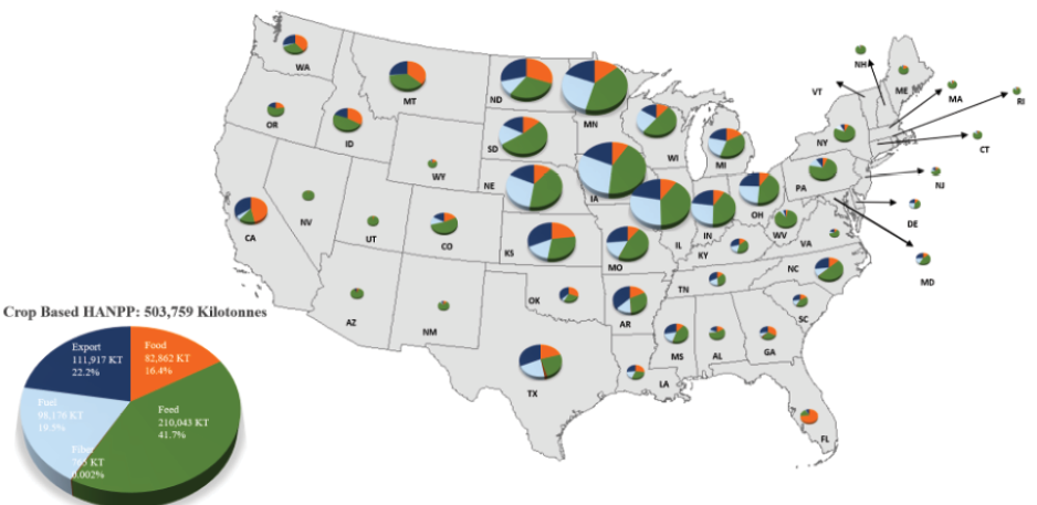
The notion that farming is environmentally and ecologically benign is widespread. It seems to harken back to an earlier, simpler era of our grandparents and great-grandparents when life was less complicated and people “lived off the land.” Certainly organic farming and local food have their merits in rebuilding some of what has been lost in the relationships food builds between people and their local environment and community. Yet in the U.S. three-fourths of all cropland grows only five crops: corn, soybeans, wheat, hay, and cotton. Of these, only wheat is used primarily for food. Figure 11.11 shows that in the U.S., livestock feed at 42 percent, exports at 22 percent, and biofuel at 20 percent all exceed food at 16 percent for allocation of crops. This is especially the case in the highly fertile Midwest, where food, mostly wheat, is an orange sliver in the large crop pies in Figure 11.11. These figures compare to 67 percent allocation to food globally. It has been calculated that shifting crop production and allocation from feed and fuel could produce food for 4 billion people. So local food markets, where I buy my fruits and vegetables when they are locally in season, are a good thing but only focus on one narrow slice of the agricultural land use pie. Clearly one way to reduce the footprint of crop production is to focus more on food.

When we use footprint analysis to measure the commitment of land and water, nitrogen, phosphorus, and carbon sinks to the agricultural enterprise, we get a picture of agriculture as a dominant consumer of renewable resources and waste sinks. The majority of grassland and savanna ecosystems worldwide have been converted to agriculture as well as nearly half of temperate deciduous forests. Over a fourth, and climbing, of tropical forests have been cleared for agriculture.

So we need to think a little harder about how to meet the challenge of agricultural sustainability. The “Solutions for a Cultivated Planet” article cited above provides five strategies, in addition to using genetic and other technologies to continue to increase yields, that can drive a more sustainable agricultural enterprise worldwide and for the U.S.

1) Stop expanding agriculture. Land clearing is the single greatest threat to biodiversity and also releases large quantities of carbon to the atmosphere that had been contained in plants and soil. Given that the most productive agricultural lands have been in production for generations, and the margin for expansion in tropical forests is both lower-productivity and high in ecosystem services and biodiversity conservation value, a clear case can be made that expanding agricultural area works against sustainability. The drainage of wetlands, our best ecosystem services packages, for crop production furthers this case against adding more land to crop production.

2) Close yield gaps. Crop yields, such as for corn in the U.S. as we saw above, have continued their remarkable climb. This is not true worldwide, however, where crop yields vary greatly. Nutrient and water limitations, lack of advanced seeds, poor management, and other factors limit yields in much of the world, especially in developing regions of Africa, parts of Latin America, and Eastern Europe. Closing the gap between possible and actual yields would reduce rural poverty and make more world regions self-sufficient.

3) Increase agricultural resource efficiency. The topic of irrigation efficiency tends not to come up in casual conversation at social gatherings. Yet getting “more crop for the drop” is an issue central to natural resource sustainability. In Chapter 3, we defined evapotranspiration as the sum of evaporation and transpiration but evaporation does nothing to produce food while transpiration is essential to power photosynthesis. Modern irrigation systems, such as drip irrigation, often led by Israeli technology, use small underground pipes to delivery water drop by drop into the root zone of crops below ground so that evaporation is minimized. Satellites and drones can monitor the greenness of crop fields over both space and time to target areas needing irrigation water and fertilizer.

Yet there are enormous efficiency gaps. Central pivot irrigation makes the Great Plains appear as a pattern of giant circles from an airplane window but is much more efficient on a calm night than on a hot windy afternoon. From there it gets worse. Unlined canals, flood irrigation over uneven fields, and other wasteful practices are surprisingly common. In the next chapter focusing on water, we’ll see how sometimes there is no incentive for farmers to invest in efficient irrigation systems.

Fertilizer applications are critical to achieving near-optimal yields, yet excessive applications are the leading source of polluted runoff. So this is a problem of getting it just right. Unfortunately, Gulf Hypoxia resulting from nitrogen runoff from the Mississippi River is not the only case of a “dead zone”; the problem is escalating worldwide, with hypoxic conditions appearing along the northern coast of Europe, in the Mediterranean, the Bay of Bengal, along the East Asian coast, and elsewhere.

Fertilizer runoff is an example of a negative externality overwhelming the denitrification capacity of watersheds, a clear case of a tragedy of the commons as we explored in Chapter 9. Providing technical assistance, eliminating subsidies for fertilizers, or even taxing or regulating them, emerge as policy tools to address this acute problem of agricultural sustainability.

4) Reducing waste. Czech-Canadian environmental scientist Vaclav Smil has analyzed the energy content of the food system and finds that less than half the calories harvested from the field are consumed by people. For every 100 calories harvested worldwide, 13 are lost postharvest, largely to pests. Another 37 are fed to livestock, with only 11 regained as meat and dairy products. An additional 17 are lost in the distribution system and households, leaving only 44 that are actually eaten by people. In the U.S., losses are even higher than the worldwide figures due to an emphasis on biofuels and livestock and high rates of food waste. Grocery stores often discard perfectly edible, but imperfect, produce that customers pass over. Expiration dates on meat and dairy products are usually too stringent encouraging households to throw away perfectly good food. Restaurants are another source of waste. We are certainly not running a tight ship even though all food carries with it a water, carbon, nitrogen and phosphorus footprint that serves no purpose if the food is not eaten . . . or is overeaten.

5)  . While we associate agriculture or farming with producing food for people, this is only partly true. Much agricultural land is devoted to producing feed for livestock, fiber products like cotton, or biofuels. In 2018, fully 40 percent of all corn grown in the U.S. was used for ethanol in gasoline, and most of the rest feeds livestock. Corn’s rotational partner, soybeans, is also largely sent to feedlots, as is the hay grown on less fertile lands.

Livestock production is a central sustainability concern. Livestock constitute over 60 percent of mammalian and a similar fraction of bird biomass on Earth. Feeding them utilizes three-fourths of global agricultural land. Cattle are specifically at issue, requiring 28 times more land, 11 times more irrigation water, 6 times more reactive nitrogen, and 5 times more greenhouse gas emissions than other forms of animal-based calories. Shifting from beef to chicken and pork could release crops sufficient to feed 357 million people; further shifting to dairy and eggs could feed 815 million people.

What I am arguing here is not that cattle are evil, but that they are qwerty. What does that mean? Look at your keyboard and on the upper left you will see this “word” spelled out. It’s not at all an efficient way to place the 26 letters of the alphabet on a keyboard—in fact, it is just the opposite. A century ago, though, this deliberately inefficient layout was used to slow down typists who would otherwise jam the keys on old typewriters. Yet when the whole world switched to computer keyboards, cellphone texting pads, and everything else we now write on in the 21st century, this layout of the letters came along for the ride as technological lock-in. It makes no sense but it’s hard to change because every day our fingers and nervous systems are getting tied into that layout as the powerful form of human capital known as habits.

Similarly, cattle were an essential tool of survival when the American frontier was extended west of the Mississippi River through the Louisiana Purchase, Mexican Cession, and Oregon Compromise. The majority of this newly acquired land is grassland with a net primary productivity that humans found a way to appropriate. While humans can’t eat grass, they can eat cattle and drink their milk and, as ruminants, cattle can eat grass. So cattle became the great tool to HANPP or colonize vast grasslands and in that context they remain a valuable and potentially sustainable element of agricultural productivity. The problems come in when the Green Revolution generated an enormous surplus of grain, especially Midwestern corn, with no obvious market. So cattle, the livestock species that was most familiar, in fact ubiquitous, became the means through which to dispose of these massive corn surpluses to produce a salable product in the form of ever more beef production. The U.S. beef cow population grew four-fold between 1939 and 1979 from 10 million to over 40 million head as hamburgers became a staple food for Americans. Notice that cattle, large animals on the order of 1,000 pounds, have a high feed conversion ratio of around 8 and up to 15 as harvested. So one cow can dispose of up to 15,000 pounds of surplus corn! This is as deliberately inefficient as the qwerty keyboard layout and has become just as locked-in.

A similar story could be told about coal, which enabled the 18th and 19th-century industrial revolution. Without coal, human civilization would not have progressed in anything approaching the rapidity that it has and, without cattle, the Western U.S., and much of South America as well, would never have been settled and brought under the influence of modern times. Anything that has been central to survival and progress for a couple of centuries is inevitably going to become a cultural icon—like the coal miner, the cowboy, the hamburger, and the beefsteak.

Yet traditional virtues such as hard work and self-reliance are not embedded in cattle and coal any more than inspired creative writing is embedded in the typewriter. An equally important virtue is to embrace a better way of doing things. So I don’t look forward to the last cow disappearing from the American farmscape, especially from uncroppable grasslands where they belong so much more than in Confined Animal Feedlot Operations (CAFOs), but I do look forward to the day when we can look back at “peak cattle” decades into the phasing out of this unsustainable practice, just as we can already look back upon “peak coal,” which occurred in 2009 (perhaps).

What is Sustainable Agriculture?

Fortunately, there are sustainable alternatives to the current system of agrochemical-intense crop production, overgrazing of grasslands, and CAFOs that globally has left 800 million people under-nourished but a billion overweight. Michael Pollan, in his widely-read critique of the U.S. agricultural and food delivery system, The Omnivore’s Dilemma, describes the Polyface Farm in Virginia, run by Joel Salatin. This grass-based farm is pastoral (rather than industrial) and biological (rather than mechanical), based on perennial (rather than annual) crop species. It is a polyculture (rather than a monoculture) relying on solar energy (rather than fossil fuels) to produce a diversified (rather than a specialized) set of products for the local (rather than the global) market. At its heart is the utilization of ecological interactions among the farm’s various species of plants and animals.

It seems the chickens eschew fresh manure so Joel Salatin waits three or four days before bringing them in—but not a day longer. That’s because the fly larvae in the manure are on a four-day cycle, he explained. “Three days is ideal. That gives the grubs a chance to fatten up nicely, the way the hens like them, but not quite long enough to hatch into flies. . . . The hens picked at the grasses, especially the clover, but mainly they were all over the cowpats, doing this frantic backward-stepping break dance with their claws to scratch apart the caked manure and expose the meaty morsels within.” . . . This is what Joel means when he says the animals do the real work around here. “I’m just the orchestra conductor, making sure everybody’s in the right place at the right time” (Pollan 2005: 212).

And make no mistake, the Polyface Farm produces a great deal of high-quality protein-rich food and does it in a manner that is cost-effective, employs somewhat more labor, and regenerates natural capital such as fertile soil rather than depleting it.

By the end of the season, Salatin’s grasses will have been transformed by his animals into some 25,000 pounds of beef, 50,000 pounds of pork, 12,000 broiler chickens, 800 turkeys, 500 rabbits, and 30,000 dozen eggs. This is an astounding cornucopia of food to draw from 100 acres of pasture, yet what is perhaps still more astounding is the fact that this pasture will be in no way diminished by the process—in fact, it will be the better for it, lusher, more fertile, even springier underfoot. Salatin’s audacious bet is that feeding ourselves from nature need not be a zero-sum proposition, one in which if there is more for us at the end of the season then there must be less for nature—less topsoil, less fertility, less life (Pollan 2005: 126).

The audacious bet of sustainable agriculture is that we are not necessarily faced with a trade-off between (a) maintaining the natural capital that makes agriculture and ecosystem services from rural landscapes possible and (b) meeting the food needs of a growing human population. We can have our cake and eat it too but only if agriculture undergoes a process of change that goes by various names like ecological intensification and permaculture. Likely, this change will only occur if the economic incentives farmers and ranchers face favor sustainable agriculture as the most profitable form of farming and if a learning culture matures where master farmers like Joel Salatin inform other farmers willing to innovate.

There are two contrasting ways of viewing this challenge. The first is an impact approach that views agriculture as a major source of pollution and a land use that removes nature. The second is a public goods approach that sees agriculture as a multifunctional enterprise that produces ecosystem services alongside food and fiber goods. These views are embedded in the structure of property rights to land and to the water that falls upon and runs through that land. The former suggests a regulatory or polluter-pays approach similar to environmental laws imposed upon other industries that use public water and air resources for waste disposal. The latter suggests a system of compensating farmers for the ecosystem services that they choose to produce from their land.

The Conservation Title of the 1985 U.S. Farm Bill set historic precedents in recognizing the importance of ecosystem services from rural landscapes. The Conservation Reserve Program (CRP) offers farmers annual payments, often in the range of $50–100 per acre per year, to replace crop production with permanent vegetative cover on highly erodible and other environmentally sensitive lands to, in essence, produce ecosystem services instead of crops. CRP has resulted in enormous reductions in soil erosion and water pollution while increasing wildlife habitat and carbon storage in soils. The program at one time had 40 million acres enrolled, an area the size of Iowa or New York, but as of this writing stands at 24 million acres as farmers have allowed their contracts to expire to take advantage of high crop prices, partly induced by biofuel subsidies. CRP thus, in a sense, leases ecosystem service provision from farmers.

The Wetland Reserve Program, initiated in the 1990 Farm Bill, offers farmers a lump sum payment in the neighborhood of $1,000 per acre to restore wetlands on cropland. As of this writing there are over two million acres enrolled in WRP. Lands damaged by major floods have been a particular focus of the program.

Organic farming exemplifies the co-production of food and ecosystem services. Separate, usually higher-priced markets for organic food have made organic farming profitable but they have also introduced a bureaucratic approach to defining what food products can legally claim the organic label, focusing on the absence of chemical fertilizers and pesticides. Note that agriculture does not need to be organic to be sustainable. In particular, modest applications of nitrogen fertilizer can increase yields without generating water quality or other problems.

These initial efforts to build programs to increase ecosystem service provision from agricultural lands are a good start. The dominant form of agricultural production in the U.S., however, remains very chemical-intensive and CAFOs continue to increase their central role in an agricultural system that is dominated by mass production of livestock and a short list of non-food crops.

Sustainable Forestry

Forests are an icon of environmentalists, some-times called “greens” for the color of tree leaves. Their opponents often refer to them derogatorily as “tree-huggers.” Some of us, myself included, enjoy spending time in the woods; others find it a lonely or even scary place.

Forests are second only to agricultural lands as a land-based resource and they share many of the same issues. Like soil, forests are natural capital that can produce provisioning services—wood as a raw material for construction, the feedstock for paper, and fuel—as well as supporting, cultural, and regulatory ecosystem services. For this reason, the primary law governing forest management in the U.S. is called the Multiple Use Sustained Yield Act. We will see that many of the dilemmas of sustainable forestry boil down to answering the question “what set of ecosystem services does the public want and how can the forest deliver them?” Or, asked differently, “among the sets of ecosystem services the forest is capable of producing, which set does the public want the most?”

Unlike agricultural lands, which are almost entirely managed privately, forests in the U.S. are more evenly split between public and private management. The U.S. Forest Service, founded by Gifford Pinchot in 1905 under the direction of President Teddy Roosevelt, manages 193 million acres, an area larger than Texas. While not all of this area is covered by trees, most of the area of the western mountain ranges is in national forests as are many of the steepest lands of the sprawling Appalachian chain. Of the 751 million acres of forest in the U.S., 44 percent is in national forests and other public lands, but the majority, 56 percent, occurs on private land.

Timber can be considered a crop but one with a long rotation of decades rather than a growing season, making it less profitable than annual crops on land where these can be grown. Forests usually generate a more abundant package of supporting, cultural, and regulatory ecosystem services than agricultural land. While soil erosion presents an ever-present danger to the value of agricultural natural capital, fire is the greatest threat to forests. Both share a concern that invasive species, pests and diseases will take over, crowding out the crops or the timber managers are trying to produce. Both also share a concern that climate change will alter the ecology to which managers have become accustomed.

Agricultural lands are not natural ecosystems; they are cultivated for specific human benefits. So also are some forests such as orchards and ornamental trees on front lawns. Forests range along a continuum of human intervention from cultivated, through managed commercial forests, through natural forests managed for fire suppression, to true wilderness.

Unlike in the tropics, the area covered by forests in the U.S. has been slowly increasing for a century. Why is this the case? Where precipitation exceeds potential evapotranspiration, as it does in the eastern half of the U.S., in the Pacific Northwest, and in the high Rocky Mountains, forests will naturally grow wherever plows, bulldozers, and fires fail to prevent it. Therefore, in humid climates, rural land that is not used for crops or grazing is nearly always forest. As the agricultural margin retreats, forests advance. Think of this historically. The pioneers headed west for land. East of the Mississippi River, most was forested land from which they would cut and burn out a farm. Many of these farms are still producing crops or livestock today but on hilly, infertile, and erosion-prone lands, the farms failed the ecological test of resiliency and the economic test of profitability. As soon as farmers stopped clearing and planting, the forests began to return. Thus the increase in forest has occurred largely due to a process of abandonment of marginal farms and natural succession. Along with forests that have been cut for timber in the past, it is often called second-growth forest in contrast to virgin or old growth forest that has not been cut in historic times. In much of the Eastern U.S., these second-growth forests continue to grow; the volume of standing timber doubled between 1960 and 2010 in an unheralded example of natural capital accumulation.

Economics of a Stored Natural Resource

Following the logic in Part II, let us consider forests first from a neoclassical economic perspective where the primary forest product is wood as a raw material. Every year that goes by, the trees are growing, adding more wood to the natural capital stock. At some point in time, however, we need to call in the lumberjacks and harvest the wood. When is the best time to do this? Figure 11.12 shows a typical growth curve over a century for trees to be used for timber. Yellow pines in the southeast may grow faster than this and Douglas firs in the northwest may grow slower but each will start off as saplings that add wood gradually, and then surge in height and girth as they mature. As they age, however, their rate of growth will slow until the maximum wood-storing capacity of an acre of forest is reached. Marketable timber is always less than the full mass of wood because twigs, roots, small branches (called ‘slash’) are not suitable for use.

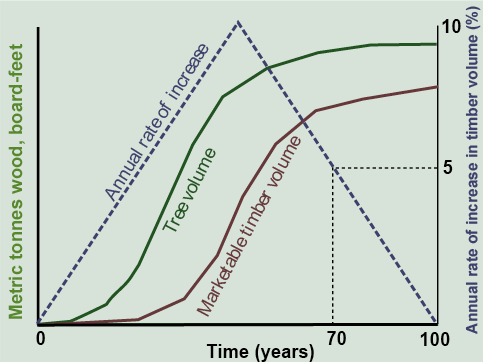
You may think that the best time to cut is when the full volume of marketable timber is reached, at 100 years in Figure 11.12 but this is not the case. If the volume of timber is increasing at a slower rate than the investment market could return, say a 5 percent annual rate of return, it is more profitable to harvest the timber and invest the profits. The optimal time to cut then becomes 70 years—30 years sooner. This also gives the next generation of trees a 30-year head start.

Over a larger area, a few tracts are being harvested while the rest continue to grow. As long as the overall increase in tree volume through growth is equal to or greater than the rate of cutting, then we can say the resource is being managed sustainably—at or below maximum sustainable yield. It’s not that simple, however, because the trees may not survive for 70 years.

The Management of Fire and other Ecological Threats

Forest fires are frightening and destructive, as an increasing number of breaking news stories has shown us. Despite expenditures of one to two billion dollars each year, forest fires on federal lands (mostly national forests) increased from an area about the size of Connecticut in 1960 to New Jersey in 2002 to larger than Maryland in 2017, including the Camp Fire that turned Paradise, CA into ashes, killing 85 people and destroying over $16 billion in property. The perception that wildfires are growing worse is clearly based in reality. A new record for a creage burned was set in 2020.

Fire is a defining characteristic of forest ecosystems. Natural fires started by lightning have always been present. Native Americans were great advocates of burning the forest to clear land for crops, to chase prey into hunters’ traps and to encourage grasslands as habitat for their prey, such as bison. Today, humans start about 90 percent of wildfires either accidentally or deliberately. Except for the wettest rainforests, such as those found along the Pacific coast north of California, most forests have a fire history that in some way has controlled their development. Pine and oak, two of the most common tree genera in the U.S., are well adapted to fire. Some pine species have seeds that only open and germinate during or after fire. Most oak saplings cannot grow in the shade of their parents; they need fire to clear a sunny spot in which they can thrive.

As a forest grows and matures, dead trees and fallen limbs on the forest floor are particularly apt to accelerate a fire started during drought conditions. Fuel gradually accumulates and, with it, the fire risk. Small ground fires can usefully remove this debris, helping to prevent large destructive fires in the future. But fire is precarious; it’s hard to predict when a change in the wind, weather, topography, or the distribution of fuel will turn a small, useful fire into a conflagration that destroys hundreds of square miles of forest or people’s homes.

Fire suppression has always been the most important mission of the U.S. Forest Service but the question of when fire is a good thing has never been settled. For most of the 20th century, the policy was to put out all forest fires as quickly as possible. This led to the accumulation of fuel, however, increasing fire risks. In recent decades, the pendulum has swung toward seeing fire as an essential tool of ecological management but when summer homes and rural residences start penetrating the forest, protecting people and their property take precedence over ecological management. Fire also releases vast quantities of carbon dioxide that are better kept out of the atmosphere, stored in wood.

Beyond fire, windstorms, invasive species, and pest outbreaks pose a danger to forests, often one that is heightened by climate change. For example, milder winters have facilitated the spread of bark beetles into the forests of the Alaskan coast, killing untold thousands of valuable spruce and cedar trees, leaving a landscape vulnerable to fire in their wake. Kudzu and Asian bittersweet vines strangle forests in the southeast. Controlling these biological invasions is often a losing battle. Fungal plagues of Asian origin wiped out two wonderful deciduous trees species—the American chestnut and the Dutch elm. Due to all of these ecological risks, the nice S-shaped growth curve presented in Figure 11.12 may never play out.

Ecosystem Services from Forests

So far, we have only been considering forests as a risky place to try to grow a sustainable supply of wood. A forest is an ecosystem that produces many other services as well. In fact, only wetlands generally produce greater ecosystem services than forests on an acre-by-acre basis. In increasing recognition of these competing demands from forests, the concept of ecosystem management was born. That is, forests need to be managed for the full suite of ecosystem services rather than wood supply alone. Table 11.1 lists these services under the four categories of supporting, provisioning, cultural, and regulatory adopted by the Millennium Ecosystem Assessment.

Table 11.1. Typical ecosystem services provided by forests.

Supporting	Provisioning	Cultural	Regulatory
photosynthesis/primary productivity	timber supply	landscape aesthetics	flood control
maintenance of biodiversity	pulp for paper	recreation	water purification
soil formation and binding	game	spiritual values	carbon storage
nutrient cycling	biofuel feedstock	hunting and gathering	pollination

So do we have to choose only one ecosystem service from this list? Of course not, because many of them are complementary—provide one and others come along with it. Can we have them all? No, because some of them are competitive—they form a trade-off. In particular, you are perhaps thinking that maximizing the timber, biofuel, and paper pulp supply competes with all the rest. That’s why we need to protect the forests. But it’s not that simple. Its a complex problem of, first, determining what ecosystem services the public wants, essentially a political exercise, and then figuring out how best to deliver them over time from the forest ecosystem, essentially a scientific and management exercise. Let’s penetrate this idea a bit deeper through some controversial resource management problems in our national forests. In each of these, look for how the problem boils down to the question: What ecosystem services does the public want and how can the forest deliver them?

The Shawnee National Forest, which contains most of the public land in Illinois, is a hunter’s paradise with waterfowl, wild turkey, and large white-tailed deer that grow fat on acorns and hickory nuts. Beneath the 80–120-foot-tall oaks and hickories, one finds slowly growing maples and beech that can tolerate the shade. In time, however, the oaks and hickories will die off, taking the mast of acorns and hickory nuts with them, leaving a maple-beech forest that is even more beautiful in the fall but that lacks the abundance of food for the game that hunters and naturalists now enjoy. In other areas, yellow pine was planted in rows decades ago, leaving a bounty of potential two-by-fours but less wildlife habitat.

Under natural conditions, raging fires opened up areas for restoration of oak and hickory, but today, such fires are suppressed to protect the significant rural population that enjoys their homes in the woods. If a return of the natural fire regime necessary to maintain the oak-hickory forest is too risky, a replacement mechanism is clear-cutting and replanting with acorns and hickory nuts. This would simulate the natural fire regime while providing high-quality wood and establishing oak and hickory forests for the rest of the century. Deer would flourish 5–20 years after the cut when abundant tree leaves are within reach. However, clear-cutting is, understandably, opposed by local environmental groups, who find the current forest structure highly aesthetic for recreational activities such as horseback riding and have a gut reaction against cutting—especially when, in the Shawnee, it generally doesn’t turn a profit. What’s your solution to the problem of what ecosystem services does the public want and how can the forest deliver them?

The most well-known forest controversy in the U.S. is the management of the northwestern forests. The issue is often painted as a conflict between jobs for lumberjacks harvesting the most profitable timber supply in the national forest system vs. the endangered northern spotted owl of the old growth forest. Is that the issue? Or is it a tug-of-war between different sets of ecosystem services?

The harvesting of old-growth timber in the once stupendous forests of the Northwest is nearly complete—only about ten percent remains—while most of the region is blanketed with second-growth forests that will start to reach maturity in coming decades. A similar cycle of the “great cut” of large old-growth trees, followed by regeneration and more sustainable management of second growth, occurred in earlier centuries in the eastern and lake states. Only now we have the Endangered Species Act that forbids federal actions that would lead to the loss of habitat of listed species.

Dependent on the old-growth environment that includes large dead trees called snags, northern spotted owls are a fine bird species that we wouldn’t want to lose to the abyss of extinction. But are they the real issue or just the point at which the teeth in the Endangered Species Act bite? Ecological studies revealed 312 plant, 149 invertebrate, 90 terrestrial vertebrate, 112 anadromous fish, and 4 resident fish species that are also dependent on the old-growth ecosystem. So the issue is far larger than the endangered northern spotted owl: it is the preservation of the forest-based natural capital that generates a suite of ecosystem services listed in Table 11.1. Of particular interest are naturally spawning salmon and a mountainous forested landscape that is second to none for its beauty and recreational opportunities. Salmon and this grand landscape symbolize the Northwest, a region many Americans have deliberately migrated to, despite the endless drizzle, just to soak it all in. The northern spotted owl doesn’t particularly symbolize these values, rather the Endangered Species Act is the most effective legal lever that people who value this suite of ecosystem services can use to protect them—and the owl is the best species to engage that law.

On the other side of the debate, timber cutting generates jobs and income and helps maintain low prices for lumber. When timber is exported as raw logs rather than as finished wood products, however, many potential jobs in wood-based industries are actualized overseas.

With these issues boiling over, the Clinton Administration negotiated the Northwest Forest Plan in 1994 applying to national forests in northern California, western Oregon, and Washington. Among other elements, the plan called for protection of old-growth forests that contain endangered species and protection of riparian corridors along streams, while vigorous timber-cutting programs of over one billion board feet per year were to continue.

Unfortunately, most observers are disappointed with the progress made under the plan. Rather, the legal requirements of the Endangered Species Act have held sway in court. There has been little active management to control fire risks or to thin maturing forests to accelerate their development of old-growth characteristics. Timber cutting and associated jobs have plummeted in a sea of red tape while profitable, value-added, wood-based industries have not developed. This disagreement over forest resource management has failed to ask, no less answer, the question “what ecosystem services does the public want and how can the forest deliver them?”

Ecosystem Services over Space and Time

Not only timber cutting, but other ecosystem services have a time and space dimension. Figure 11.13 uses the same axes as Figure 11.12 but charts how certain ecosystem services develop as the forest grows. Forests are excellent at filtering water as it seeps through the leaves, stems, and roots, and at controlling floods by transpiring and storing water. These services become available early on, as soon as the forest forms a dense canopy of saplings. Different forest wildlife species thrive at different periods. The northern spotted owl is a creature of old growth but deer enjoy the early phase when more leaves grow within reach. (Recall the example of the Tongass National Forest from Chapter 10.) Most people find mature and old-growth forests with large trees and limited undergrowth more aesthetically pleasing, even cathedral-like, than the dense, nearly impenetrable brush of a newly restored forest. So as a forest matures, its suite of ecosystem services evolves with it.

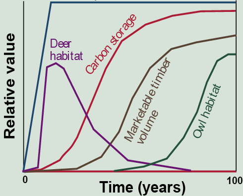
Carbon storage, an increasingly critical forest service, is coincident with the volume of wood in the growing forest, about 45 percent by weight in trunks and leaves alike. Researchers from Woods Hole Research Center in Massachusetts showed that, prior to 1945, the U.S. landscape was a source of carbon emissions but that, since 1945, it has become a substantial carbon sink. Largely due to fire suppression and forest growth on abandoned farmlands, growing U.S. forests are offsetting over 10 percent of U.S. carbon emissions from fossil fuels. This lends another angle to the long debate over fire suppression since the accumulation of woody debris removes carbon from the atmosphere, while burning releases it, as does decay. Perhaps deadwood could be collected from forest floors to replace a bit of coal, thus killing the renewable energy, fire management, and climate change birds with one stone.

Space also matters. The services of water purification and flood control are best provided by forests hugging streams—the riparian zone. Biodiversity can be maximized by interspersing forest tracts of different ages, thus providing a variety of habitats but some species require large contiguous tracts of old growth. All of these intersecting goals calls for a new paradigm.

Ecosystem Management

Ecosystem management is a concept developed in the 1990s by a coalition of scientists from academia and federal agencies, with special reference to management of public lands and forests. It arose partly from the failure of management focused on wood supply and fire suppression on the one hand, restrained by the Endangered Species Act (which only kicks in when species are about to disappear) on the other. Done properly, ecosystem management is a process to answer the question we have posed: “What ecosystem services does the public want and how can the forest (or landscape) deliver them?” It also acknowledges how difficult that can be. First, different segments of the public want different things. Some want to buy wood cheap, others want to protect their favorite recreational spot, others want to save species from extinction or preserve the aesthetics of the forest in its natural state. Working this all out is a terribly difficult, though not impossible, political and economic task.

Second, ecosystems are complex systems that are unpredictable and only partly understood. Fires, floods, droughts, pest outbreaks, wind-storms, exotic species invasions, human mismanagement—these disturbances all occur, and the ecosystem must be able to either resist them, or more likely be resilient to them.

For this reason, resilience is a critical concept in ecosystem management. What does it mean? If I say that you are resilient, it means that when a hardship comes—illness, injury, loss of a loved one, financial loss, a damaging addiction—you are able to rebound in a way that maintains your vigor and positive direction. For an ecosystem, it means that it can withstand disturbance or exogenous shocks and still maintain its fundamental ecosystem functions and dynamics—though it will never return to its original state. Ecologists are still working out what makes an ecosystem resilient but biodiversity almost certainly helps because if one species suffers a major setback, another can take its place in the food web and in the performance of essential functions like decomposition or nutrient cycling. Ecological resilience, and therefore biodiversity, is thus central to natural resources sustainability.

All of this entails a measure of humility as well. We only partly understand the complexity of ecosystems and cannot always predict how they will respond if humans do X or Y. Like in medicine, we can at least record the management measures that were taken and the results that occurred. Then we can adjust the treatment, if necessary, and again record the results. In the natural resources field, this is called adaptive management. It is distinct from planning because to develop and implement a plan, two prerequisites must be present: the planner has the political authority to implement the plan and the results of management actions are predictable. Yet these two prerequisites are rarely met. Adaptive management—learning as you go through observation and experimentation—thus goes hand-in-hand with ecosystem management as the best ideas we currently have for managing our forests and other landscapes sustainably.

Analyzing Ecosystem Services from Rural Landscapes

On largely privately-owned rural landscapes, the most common type in the U.S., especially between the Rocky Mountains and the eastern seaboard cities, agricultural production co-mingles with semi-natural land uses. Aggregately, these landscapes generate both private provisioning and public ecosystem services. An example will help illustrate.

The land that forms Big Creek, near my former home at Southern Illinois University, is divided into a large number of privately-held land units or farms. In selecting land uses, say between crops, pasture and forest, each farmer responds not to the watershed-scale performance, but to the performance of his or her own farm, given the characteristics of the land they have to work with and the policies and economic conditions that apply to it.

Figure 11.14a, for example, shows that, in humid climates where crops and forests will grow without irrigation, we find that crops are most profitable on flat, fertile, well-drained land. Producing crops is expensive, however, and profits fall toward zero on marginal land that may be less fertile, a bit hilly, or frequently flooded. These lands are better suited to pasture, which is less profitable, but also less costly. On even less productive land—hilly, infertile, rocky, or perennially wet—forests remain or are allowed to regenerate. So the land use map of a watershed tends to be well-organized with crops on the most fertile, forests on the least fertile, and pastures on the intermediate land from the standpoint of agricultural productivity. This occurs not by a central plan, like on a National Forest, but by each farmer or landowner doing what they see as best on their own parcels. In more densely populated countries, such as many in Asia, farmers will push crop production onto even more marginal land using terraces and other labor-intensive practices—usually at the expense of forests. This also occurs in the U.S., as shown in Figure 11.14b, when crop prices are high, such as when large volumes of corn are used to produce ethanol.

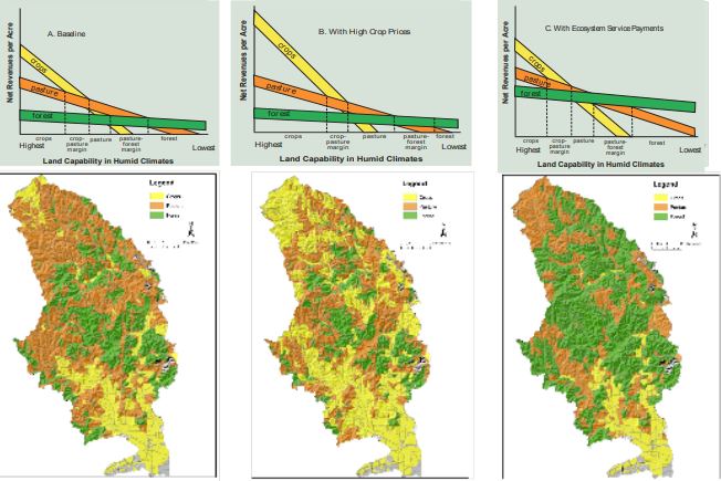
Forests produce greater ecosystem services per acre than pasture; pasture produces more than cropland. If farmers were actually paid for these services, say through the Conservation Reserve Program or carbon credits, it would increase the profitability of forests the most and crops the least. This would encourage forests on what had been pastures and pastures on what had been cropland (Figure 11.14c). Crop food production would decrease a bit but ecosystem service provision would increase greatly on an evolving land use map.

In the more arid landscapes characteristic of much of the western U.S., where rainfall is insufficient to support crops or forests, we instead have a landscape of irrigated crops, on the most fertile lands where water can be obtained, and rangeland where it cannot. Where rainfall is insufficient to maintain even grazing, there is the nonagricultural desert.

As we view the rural landscape from our windshield while driving, aerial photographs, or satellite images, we are looking at a system that is organized from below—parcel-by-parcel—rather than from above in accordance with a plan. This can leave the rural landscape fragmented. Large blocks of forest are broken up by roads and farms. Large areas of wetlands or riparian ribbons along rivers are broken into remnants. This impacts biodiversity greatly, favoring edge species and species that adapt well to human-modified environments over wild species that require large areas of undisturbed forest or other natural habitats.

Land use and land cover change has rapidly emerged as a science, where changes can not only be monitored through technologies like remote sensing but even predicted using spatial and economic models. In this manner, the changes in the landscape of, say, an increase in demand for biofuels, or a shift away from eating meat, or a market for carbon, can be understood. The implications of this new map on ecosystem service provision and biodiversity can also be examined, if rarely predicted with precision. In this way, a signal can be found connecting, say, the consumption of burgers at fast food restaurants, with the fate of endangered species in the Amazon, or, as we saw in Chapter 8 on industrial ecology, subsidies for the production of biofuels for cars with the storage of carbon in forests and soils.

This discussion of land resources and how to manage them sustainably has now become the longest chapter in this text, and yet we’ve only scratched the surface. Consider it an appetizer, one that brings you to the table for the main course.

Further Reading

Christensen, N. et al. 1996. The Report of the Ecological Society of America Committee on the Scientific Basis for Ecosystem Management. Ecological Applications 6(3): 665–691.

Foley, J, et al. 2011. Solutions for a cultivated planet. Nature. doi:10.1038/nature10452.

Pollan, M., 2006. The Omnivore’s Dilemma: A Natural History of Four Meals. Penguin Press.

Media Attributions

Figure 11.1 © Christopher Lant is licensed under a CC BY-NC-SA (Attribution NonCommercial ShareAlike) license Figure 11.2 © United States Federal Government is licensed under a Public Domain license Figure 11.3 © GISGeography is licensed under a All Rights Reserved license. Used with permission Figure 11.4 © GISGeography is licensed under a All Rights Reserved license. Used with permission Figure 11.5 © USGS is licensed under a Public Domain license Figure 11.6 © Multi-Resolution Land Characteristics Consortium is licensed under a Public Domain license Figure 11.7 © Jonathan A. Foley, et al. is licensed under a All Rights Reserved license Figure 11.8 © Christopher Lant is licensed under a CC BY-NC-SA (Attribution NonCommercial ShareAlike) license Figure 11.9 © Christopher Lant, adapted from Tilman, et al., 2002 is licensed under a CC BY-NC-SA (Attribution NonCommercial ShareAlike) license Figure 11.10 © Christopher Lant, adapted from Tilman et al., 2002 is licensed under a CC BY-NC-SA (Attribution NonCommercial ShareAlike) license Figure 11.11 © Christopher Lant, et al. is licensed under a All Rights Reserved license Figure 11.12 © Christopher Lant is licensed under a CC BY-NC-SA (Attribution NonCommercial ShareAlike) license Figure 11.13 © Christopher Lant is licensed under a CC BY-NC-SA (Attribution NonCommercial ShareAlike) license Figure 11.14 © Christopher Lant is licensed under a CC BY-NC-SA (Attribution NonCommercial ShareAlike) license