Presenting quantitative research results in a visual format can be a quick and effective way to show what you’ve found. However, just like statistics broadly, charts, graphs, and tables can also be used maliciously to manipulate how data are understood. In all data presentation, you should strive to make the results clear, easy to understand, and above all, honest. Most of the time, simpler is better, and it’s always worth checking your visualization with other people to see if they make the same interpretations you do or if there is more you can do to simplify and clarify your results.

Pie charts are infamous – they are a beloved favorite of many a novice data analyst, which is both a strength and a weakness. If you need to present proportional data, a pie chart, in which a circle is divided into “slices” that are proportional to the size of the category they represent, can be simple. If you choose to use a pie chart, be certain that the slices are accurately representing their proportion (sometimes tricky analysts will double – or more – a given slice to emphasize it, even if it is only a small numerical proportion of the pie), that all the slices add up to 100%, and that each slice is accurately labeled and can easily be differentiated from the others, hopefully with more than just color – using fill textures can help with this, or labeling the slices directly.

As an example, look at the pie chart below.

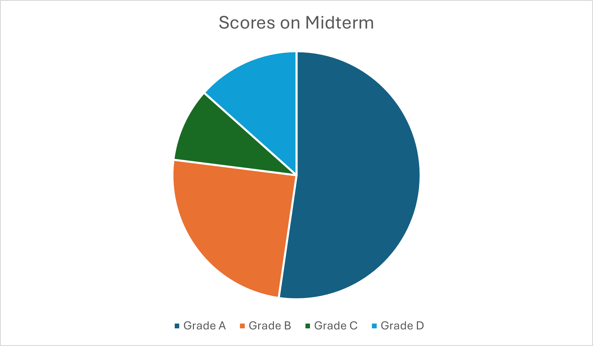
This is hypothetical grades on a midterm exam. This chart tells us a couple things: there were more A grades than not, but we can’t tell exactly how much more of the class scored an A versus another grade. We also might have trouble distinguishing the slices from each other using just color and a legend apart from the pie – even if you don’t have a color blindness condition, differentiating similar colors can be a challenge, or if you’ve printed out the page with black-and-white printing, you might run into this too!

Let’s try another version of the same pie chart:

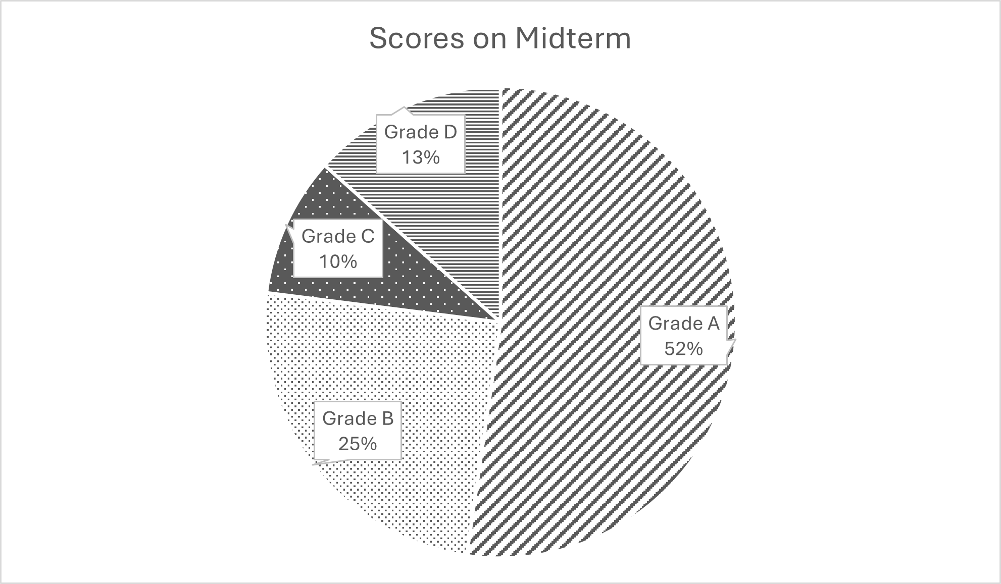
In this version, a few things have changed: the slices are now distinguishable by fill texture, each slice bears a label directly on the slice with both the name of the category and the percentage value of the category. This chart is not perfect, and no single chart will likely be perfect for every situation. If you know you’ll be using the chart in high-contrast colors, for example on a poster presentation, then you might elect to use color instead of texture. Some charts can be published on webpages where each slice can be clicked for more information, so maybe you don’t need all the labeling information initially. As with all research dissemination (which we’ll talk more about later), you must consider your audience, goals, and context of the research presentation to decide how best to show what you’ve found. A pie chart is a good choice for some contexts.

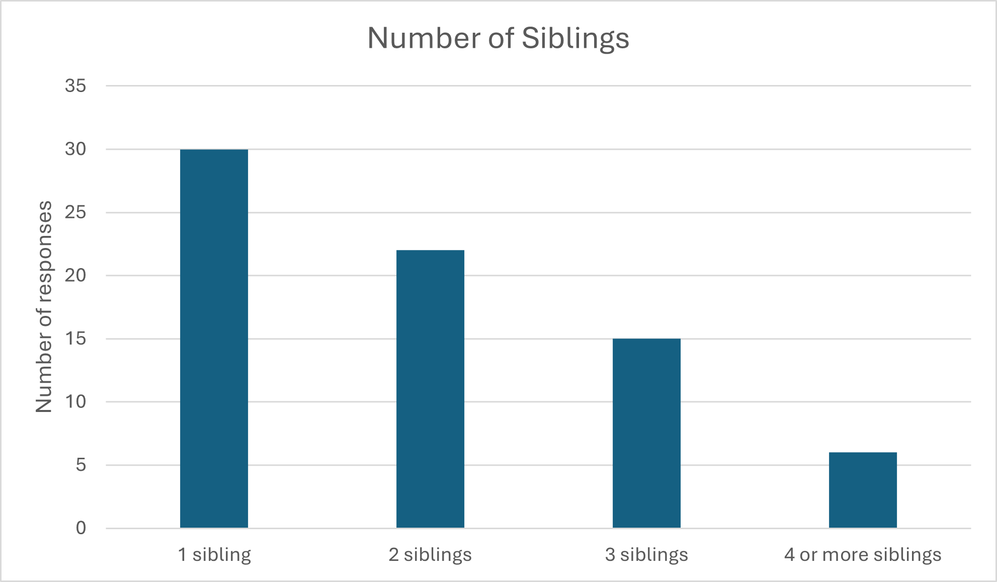
Bar graphs and their relatives, such as column charts and line charts, are the quintessential data visualization for most variables. The basic idea can work for all types of variables, from nominal to ratio, and have many variations to suite specific needs. At the core, the bar graph uses one axis, usually the X axis (horizontal, usually placed along the bottom of the graph) to name the categories or values of the independent variable (x). If you’re showing the value of something over time, “time” is likely going to be the X axis. The Y axis (vertical) then runs along the side (usually left side) of the graph, and shows the value of the dependent (y) variable or, if you’re using a bar graph simply to show a univariate distribution, it will be the count or percentage of the response. For example, see the bar graphs below, each showing fictional data for various outcomes of interest in a hypothetical study of oldest siblings. In the chart below, we’ve asked our hypothetical respondents how many siblings they have. Since one of the inclusion criteria of this study is that they have at least one sibling, no only children are represented here. Instead, we see that the most common response, 30 of our 72 respondents, was 1 sibling, with numbers decreasing with each additional sibling.

You’re probably familiar with histograms as a data visualization tool. Histograms have the same basic principle of a univariate bar graph like the one above, but they are used for continuous data (data that are not in categories). Instead of listing each response value, like we did above, we need to “bin” the continuous data into groups that can allow us to see the distribution of the results. Let’s take a variable like the age gap between our respondent and their next youngest sibling (for those with younger siblings). We’ll measure it in months, and bin those months in sets of 18. In this case, we have 71 responses because we took out two respondents who are twins.

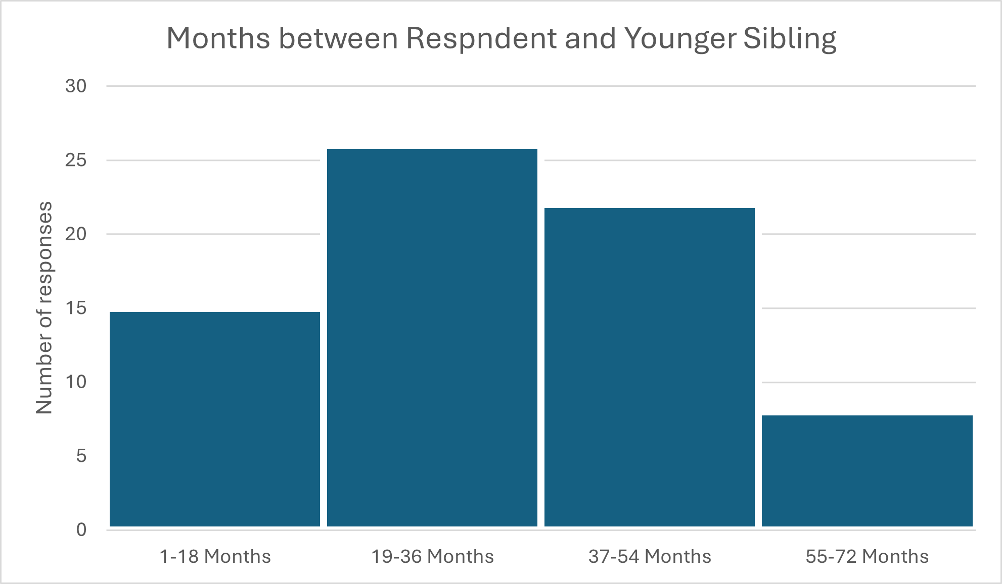
From the chart, we can see that most respondents are more than 1.5 years but less than 3 years older than their next sibling. We’d probably want more statistics on this (a mean value would be illuminating) but this is a pretty good start to understanding what our data contain.

Bar charts, and their close cousin, the line chart, can also be used for looking at change over time. For example, if we wanted to see how sibling closeness changed in the months before and after a “sibling night” event meant to enhance sibling relationships, we could chart something like this:

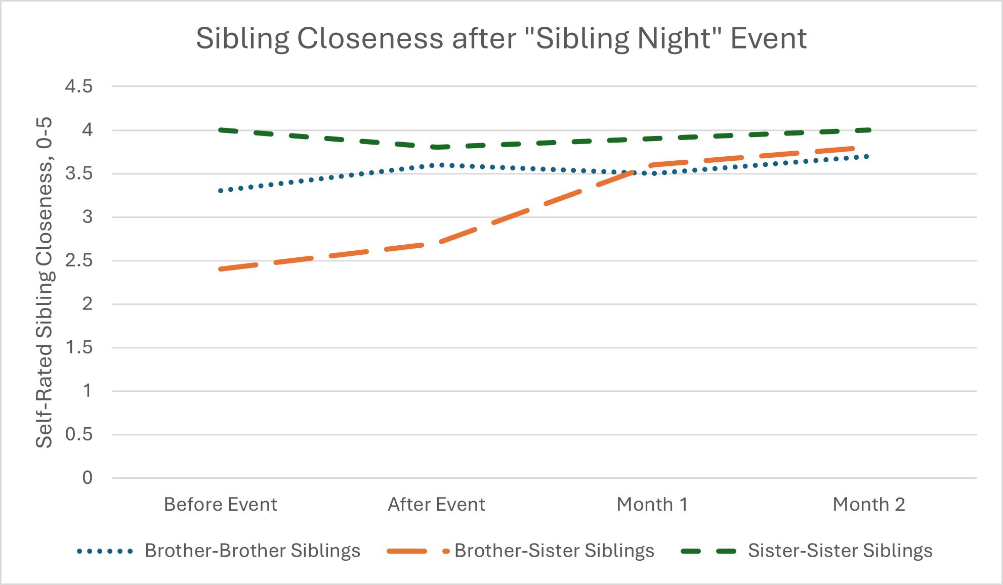
On this chart, you can see that we’ve actually included three groups, which makes this a tri-variate chart because in addition to looking at self-rated closeness and time, we’re also looking at how sibling gender composition might play a role.

Is a line or bar better? In general, lines are good for continuous variables, and bars are a better choice for categorical ones. This is one of those times when showing the graph to someone to see if they can intuitively read the data or if they have questions can be important. In general, a graph should be able to stand on its own and be interpretable with the graph and caption, without having to refer to additional text.

Scatterplots are excellent for visualizing how two variables interact – this is often the first step towards understanding correlations, which we’ll describe more in the next section. A scatterplot uses the same principles of a bar chart, with an X axis along the bottom and a Y axis along the side, and then “plots” each value in the dataset at the appropriate level of X and Y. You’ll get something like this chart, which plots the hypothetical values of sibling rivalry against self-esteem for about half our hypothetical sample:

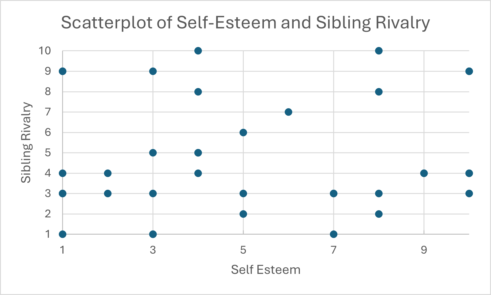
Doesn’t look like there’s much going on from the scatterplot, but we’d need to calculate a correlation to know for sure. Let’s look at the next section to learn how to do that!