"

Experimental Designs

What Makes a Study an Experiment?

We may hear the word experiment throwing around anytime someone talks about “testing” or being “scientific.” The confusion is perhaps understandable; experiments are one of the most classic research designs and are immensely useful for many fields and questions. However, it’s unfair to call just anything an experiment, as true experiments and their close cousins, such as quasi-experiments, have unique qualities that should be appreciated for what they are but not applied where they don’t fit. You need to be able to pick a true experiment out from the fakes and identify why it’s really an experiment (or not).

Experiments are an excellent data collection strategy for scientists wishing to observe the effects of a clinical intervention or social program. Understanding what experiments are and how they are conducted is useful for all social scientists, whether they plan to use this methodology or simply understand findings of experimental studies. An experiment is a method of data collection designed to test hypotheses under controlled conditions.

Experiments have a long and important history in social science. Behaviorists such as John Watson, B. F. Skinner, Ivan Pavlov, and Albert Bandura used experimental designs to demonstrate the various types of conditioning. Using strictly controlled environments, behaviorists were able to isolate a single stimulus as the cause of measurable differences in behavior or physiological responses. The foundations of social learning theory and behavior modification are found in experimental research projects. Moreover, behaviorist experiments brought psychology and social science away from the abstract world of Freudian analysis and towards empirical inquiry, grounded in real-world observations and objectively defined variables. Experiments are used at all levels of social inquiry, including agency-based experiments that test therapeutic interventions and policy experiments that test new programs.

Several kinds of experimental designs exist. In general, designs that are true experiments contain three key features: independent and dependent variables, pretesting and posttesting, and experimental and control groups. In a true experiment, the effect of an intervention is tested by comparing two groups. One group is exposed to the intervention (the experimental group, also known as the treatment group) and the other is not exposed to the intervention (the control group).

In some cases, it may be immoral to withhold treatment from a control group within an experiment. If you recruited two groups of people with severe addiction and only provided treatment to one group, the other group would likely suffer. For these cases, researchers use a comparison group that receives “treatment as usual,” but experimenters must clearly define what this means. For example, standard substance abuse recovery treatment involves attending twelve-step programs like Alcoholics Anonymous or Narcotics Anonymous meetings. A substance abuse researcher conducting an experiment may use twelve-step programs in their comparison group and use their experimental intervention in the experimental group. The results would show whether the experimental intervention worked better than normal treatment (or “business-as-usual”), which is useful information. However, using a comparison group is a deviation from true experimental design and is more closely associated with quasi-experimental designs.

Importantly, participants in a true experiment need to be randomly assigned to either the control or experimental groups. Random assignment uses a random process, like a random number generator, to assign participants into experimental and control groups (this is not “I feel like you should go with this group” or letting participants choose to be in one group or the other). Random assignment is important in experimental research because it helps to ensure that the experimental group and control group are comparable and that any differences between the experimental and control groups are due to random chance. We will address more of the logic behind random assignment later.

In an experiment, the independent variable is the intervention being tested. In family science and related fields, this could include a therapeutic technique, a prevention program, or access to some service or support. Social science research may also have a stimulus rather than an intervention as the independent variable, meaning that instead of participating in some program or intervention, the difference between the experimental and control groups is something else the treatment group is given that the control group is not – a stressful prompt, for example, or a video of a specific kind of interaction. We don’t see a lot of these examples in family science, but they do exist!

The dependent variable is usually the intended effect of the researcher’s intervention. If the researcher is testing a new therapy for individuals with binge eating disorder, their dependent variable may be the number of binge eating episodes a participant reports. The researcher likely expects their intervention to decrease the number of binge eating episodes reported by participants. Thus, they must measure the number of episodes that occurred before the intervention (the pretest) and after the intervention (the posttest).

Let’s put these concepts in chronological order to see how an experiment runs from start to finish. Once you’ve collected your sample, you’ll need to randomly assign your participants to the experimental group and control group. Then, you will give both groups your pretest, which measures your dependent variable, to see what your participants are like before you start your intervention. Next, you will provide your intervention, or independent variable, to your experimental group. Keep in mind that many interventions take a few weeks or months to complete, particularly therapeutic treatments. Finally, you will administer your posttest to both groups to observe any changes in your dependent variable. Together, this is known as the classic experimental design and is the simplest type of true experimental design. All of the designs we review in this section are variations on this approach. The figure below visually represents these steps.

This image illustrates the basic structure of an experimental research design using a step-by-step arrow flow. Each step represents a key phase in conducting an experiment: Sampling – Selecting participants for the study. Assignment – Randomly or non-randomly assigning participants to groups (e.g., treatment vs. control). Pretest – Measuring baseline data before the intervention. Intervention – Applying the treatment or condition being studied. Posttest – Measuring outcomes after the intervention to assess its effect. This sequence helps researchers determine whether changes in the posttest are attributable to the intervention.o objectives use verbs like apply, demonstrate, perform, practice, create, or evaluate?

Steps in classic experimental design

An interesting example of experimental research can be found in Shannon K. McCoy and Brenda Major’s (2003) [1] study of peoples’ perceptions of prejudice. In one portion of this multifaceted study, all participants were given a pretest to assess their levels of depression. No significant differences in depression were found between the experimental and control groups during the pretest. Then, participants in the experimental group were asked to read an article suggesting that prejudice against their own racial group is severe and pervasive, while participants in the control group were asked to read an article suggesting that prejudice against a racial group other than their own is severe and pervasive. Clearly, their independent variables were not interventions or treatments for depression, but were stimuli designed to elicit changes in people’s depression levels. Upon measuring depression scores during the posttest period, the researchers discovered that those who had received the experimental stimulus (the article citing prejudice against their same racial group) reported greater depression than those in the control group. This is just one of many examples of social scientific experimental research.

In addition to classic experimental design, there are two other ways of designing experiments that are considered to fall within the purview of “true” experiments (Babbie, 2010; Campbell & Stanley, 1963). [2] The posttest-only control group design is almost the same as classic experimental design, except it does not use a pretest. Researchers who use posttest-only designs want to eliminate testing effects, in which a participant’s scores on a measure change because they have already been exposed to it. If you took multiple SAT or ACT practice exams before you took the final one whose scores were sent to colleges, you’ve taken advantage of testing effects to get a better score. Considering the previous example on racism and depression, participants who are given a pretest about depression before being exposed to the stimulus would likely assume that the intervention is designed to address depression. That knowledge can cause them to answer differently on the posttest than they otherwise would. Please do not assume that your participants are oblivious. More likely than not, your participants are actively trying to figure out what your study is about.

In theory, if the control and experimental groups have been randomly determined and are therefore comparable, then a pretest is not needed. However, most researchers prefer to use pretests so they may assess change over time within both the experimental and control groups. Researchers who want to account for testing effects and additionally gather pretest data can use a Solomon four-group design. In the Solomon four-group design, the researcher uses four groups. Two groups are treated as they would be in a classic experiment—pretest, experimental group intervention, and posttest. The other two groups do not receive the pretest, though one receives the intervention. All groups are given the posttest. The Table below illustrates the features of each of the four groups in the Solomon four-group design. By having one set of experimental and control groups that complete the pretest (Groups 1 and 2) and another set that does not complete the pretest (Groups 3 and 4), researchers using the Solomon four-group design can account for testing effects in their analysis.

Solomon four-group design
Pretest Stimulus Posttest
Group 1 X X X
Group 2 X X
Group 3 X X
Group 4 X

Solomon four-group designs are challenging to implement because they are time-consuming and resource-intensive. Researchers must recruit enough participants to create four groups and implement interventions in two of them. Overall, true experimental designs are often difficult to implement in a real-world practice environment. Additionally, it may be impossible to withhold treatment from a control group or randomly assign participants in a study. In these cases, pre-experimental and quasi-experimental designs can be used, however the differences in rigor from true experimental designs leave their conclusions more open to critique.

So, what is an Experiment?

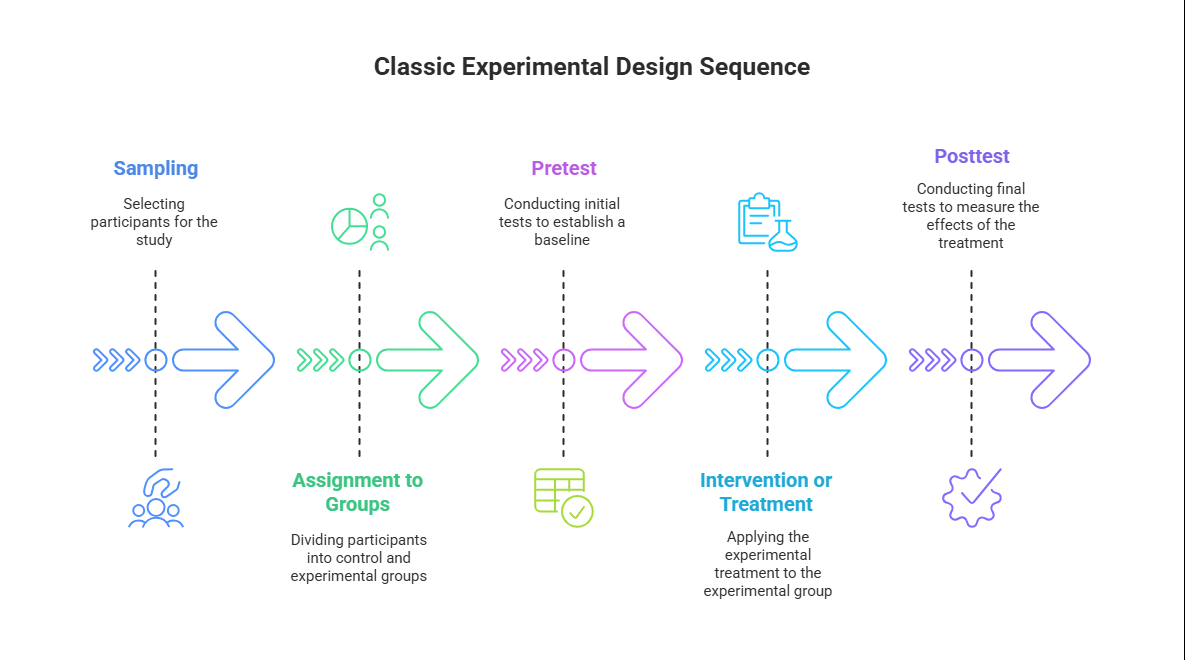
As we’ve just discussed, an experiment is a type of study designed specifically to answer the question of whether there is a causal relationship between two variables. In other words, whether changes in an independent variable cause a change in a dependent variable. Experiments have two fundamental features. The first is that the researchers manipulate, or systematically vary, the level of the independent variable. The different levels of the independent variable are called conditions. Let’s look at a specific study for an example. Pepin’s 2019 study, titled Beliefs about Money in Families: Balancing Unity, Autonomy, and Gender Equality is a great example of an experimental study that used stimuli to test the effect of certain information on beliefs. In this case, the manipulation had to do with the characteristics of a fictional couple (presented in a small story or description, called a vignette), and the outcome was how respondents felt the fictional couple should pool their money – or alternatively, if the respondents felt the couple should keep their money separate or in some combination of pooled and separate accounts. In this study, there were four independent variables, with multiple conditions in each: relationship status (with the conditions of married or cohabiting), parental status (with conditions of parents or not parents), relationship duration (3 years or 7 years), and relative earnings (equal earners, man earns more, or woman earns more). There was thus a total of 24 different scenarios that could be tested with all conditions considered; respondents each only received one scenario to rate their feelings on shared or separate money.

The second fundamental feature of an experiment is that the researcher controls, or minimizes the variability in, variables other than the independent and dependent variable. These other variables are called extraneous variables. In Pepin’s study, all respondents received the same survey in the same mode (online), with the only difference being the specific couple scenario they received, assigned randomly. Note that other details of the couple were the same for each respondent: the names of the man and woman were held steady (and by extension, the gender composition and assumed race), the ages, and the order of description was all the same for each scenario – the only differences between each vignetter were the independent variables. Notice that although the words manipulation and control have similar meanings in everyday language, researchers make a clear distinction between them. They manipulate the independent variable by systematically changing its levels and control other variables by holding them constant.

Let’s Break it Down

Show

Extraneous Variables

In simple terms:

Extraneous variables are outside factors that you’re not trying to study—but they could still affect the results if you’re not careful.

Example:

A researcher wants to know if classroom noise affects how well students do on a math test.

  • Independent variable = Level of noise in the classroom

  • Dependent variable = Test scores

But…

One group of students is being tested in the morning, and the other in the afternoon.
Or one group was tested in a room with a noxious smell and the other group didn’t have the smell in the room.

Those things—time or smell—are extraneous variables.
They aren’t part of the study, but they could still affect test scores and confuse the results.

* This image was created using ChatGPT; however, the concept, design direction, and creative vision were conceived by Dr. Knight


Manipulation of the Independent Variable

Again, to manipulate an independent variable means to change its level systematically so that different groups of participants are exposed to different levels of that variable (including any vs. none if that is appropriate), or the same group of participants is exposed to different levels at different times. For example, to see whether expressive writing affects people’s health, a researcher might instruct some participants to write about traumatic experiences and others to write about neutral experiences. As discussed earlier in this chapter, the different levels of the independent variable are referred to as conditions, and researchers often give the conditions short descriptive names to make it easy to talk and write about them. In this case, the conditions might be called the “traumatic condition” and the “neutral condition.”

Notice that the manipulation of an independent variable must involve the active intervention of the researcher. Comparing groups of people who differ on the independent variable before the study begins is not the same as manipulating that variable. For example, a researcher who compares the health of people who already keep a journal with the health of people who do not keep a journal has not manipulated this variable and therefore has not conducted an experiment. This distinction is important because groups that already differ in one way at the beginning of a study are likely to differ in other ways too. For example, people who choose to keep journals might also be more conscientious, more introverted, or less stressed than people who do not. Therefore, any observed difference between the two groups in terms of their health might have been caused by whether or not they keep a journal, or it might have been caused by any of the other differences between people who do and do not keep journals. Thus, the active manipulation of the independent variable is crucial for eliminating potential alternative explanations for the results.

Of course, there are many situations in which the independent variable cannot be manipulated for practical or ethical reasons and therefore an experiment is not possible. For example, whether or not people have a significant early illness experience cannot be manipulated, making it impossible to conduct an experiment on the effect of early illness experiences on the development of hypochondriasis. This caveat does not mean it is impossible to study the relationship between early illness experiences and hypochondriasis—only that it must be done using nonexperimental approaches. 

Independent variables can be manipulated to create two conditions and experiments involving a single independent variable with two conditions is often referred to as a single factor two-level design. However, sometimes greater insights can be gained by adding more conditions to an experiment. When an experiment has one independent variable that is manipulated to produce more than two conditions it is referred to as a single factor multi level design. If even more variables are added, we can begin to write out the design by providing the number of conditions for each independent variable. In the example above from Pepin (2019), we would call this a 2 x 2 x 2 x 3 factorial design, because it had four independent variables, the first three of which had two conditions, and the fourth of which had three conditions.

Control of Extraneous Variables

As we have seen previously, an extraneous variable is anything that varies in the context of a study other than the independent and dependent variables. In an experiment on the effect of expressive writing on health, for example, extraneous variables would include participant variables (individual differences) such as their writing ability, their diet, and their gender. They would also include situational or task variables such as the time of day when participants write, whether they write by hand or on a computer, and the weather. Extraneous variables pose a problem because many of them are likely to have some effect on the dependent variable. For example, participants’ health will be affected by many things other than whether or not they engage in expressive writing. This influencing factor can make it difficult to separate the effect of the independent variable from the effects of the extraneous variables, which is why it is important to control extraneous variables by holding them constant whenever possible, and by randomizing groups so that variables that cannot be directly controlled can be distributed.

Extraneous variables make it difficult to detect the effect of the independent variable in two ways. One is by adding variability or “noise” to the data. Imagine a simple experiment on the effect of mood (happy vs. sad) on the number of happy childhood events people are able to recall. Participants are put into a negative or positive mood (by showing them a happy or sad video clip) and then asked to recall as many happy childhood events as they can. The two leftmost columns of the Table below show what the data might look like if there were no extraneous variables and the number of happy childhood events participants recalled was affected only by their moods. Every participant in the happy mood condition recalled exactly four happy childhood events, and every participant in the sad mood condition recalled exactly three. The effect of mood here is quite obvious. In reality, however, the data would probably look more like those in the two rightmost columns of the Table. Even in the happy mood condition, some participants would recall fewer happy memories because they have fewer to draw on, use less effective recall strategies, or are less motivated. And even in the sad mood condition, some participants would recall more happy childhood memories because they have more happy memories to draw on, they use more effective recall strategies, or they are more motivated. Although the mean difference between the two groups is the same as in the idealized data, this difference is much less obvious in the context of the greater variability in the data. Thus one reason researchers try to control extraneous variables is so their data look more like the idealized data in Table 5.1, which makes the effect of the independent variable easier to detect (although real data never look quite that good).

Hypothetical Noiseless Data and Realistic Noisy Data
Idealized “noiseless” data Realistic “noisy” data
Happy mood Sad mood Happy mood Sad mood
4 3 3 1
4 3 6 3
4 3 2 4
4 3 4 0
4 3 5 5
4 3 2 7
4 3 3 2
4 3 1 5
4 3 6 1
4 3 8 2
M = 4 M = 3 M = 4 M = 3

One way to control extraneous variables is to hold them constant. This technique can mean holding situation or task variables constant by testing all participants in the same location, giving them identical instructions, treating them in the same way, and so on. It can also mean holding participant variables constant. For example, many studies of language limit participants to right-handed people, who generally have their language areas isolated in their left cerebral hemispheres. Left-handed people are more likely to have their language areas isolated in their right cerebral hemispheres or distributed across both hemispheres, which can change the way they process language and thereby add noise to the data.

In principle, researchers can also control extraneous variables by limiting participants to one very specific category of person, such as 20-year-old, heterosexual, female, right-handed psychology majors. The obvious downside to this approach is that it would lower the external validity of the study—in particular, the extent to which the results can be generalized beyond the people actually studied. For example, it might be unclear whether results obtained with a sample of younger heterosexual women would apply to older homosexual men. In many situations, the advantages of a diverse sample (increased external validity) outweigh the reduction in noise achieved by a homogeneous one.

The second way that extraneous variables can make it difficult to detect the effect of the independent variable is by becoming confounding variables. A confounding variable is an extraneous variable that differs on average across levels of the independent variable (i.e., it is an extraneous variable that varies systematically with the independent variable). For example, in almost all experiments, participants’ intelligence quotients (IQs) will be an extraneous variable. But as long as there are participants with lower and higher IQs in each condition so that the average IQ is roughly equal across the conditions, then this variation is probably acceptable (and may even be desirable). What would be bad, however, would be for participants in one condition to have substantially lower IQs on average and participants in another condition to have substantially higher IQs on average. In this case, IQ would be a confounding variable.

Let’s Break it Down

Show

Confounding Variable

In simple terms:

A confounding variable is something extra that affects both the cause and the effect you’re studying. It makes it hard to tell if the results are really caused by the factor you’re testing, or by this other hidden factor.

Example:

A researcher wants to study if screen time (how much time teens spend on phones or computers) affects their grades.

  • Independent variable = Screen time

  • Dependent variable = Academic performance (grades)

But… what if students who spend more time on screens also sleep less?

Now the researcher can’t tell if bad grades are due to screen time or because the students are tired from lack of sleep.

 In this case, sleep is a confounding variable—it’s linked to both screen time and grades, and it could be the real reason for the drop in performance.

* This image was created using ChatGPT; however, the concept, design direction, and creative vision were conceived by Dr. Knight


To confound means to confuse, and this effect is exactly why confounding variables are undesirable. Because they differ systematically across conditions—just like the independent variable—they provide an alternative explanation for any observed difference in the dependent variable. Above, we talked about a hypothetical study in which participants in a positive mood condition scored higher on a memory task than participants in a negative mood condition. But if IQ is a confounding variable—with participants in the positive mood condition having higher IQs on average than participants in the negative mood condition—then it is unclear whether it was the positive moods or the higher IQs that caused participants in the first condition to score higher. One way to avoid confounding variables is by holding extraneous variables constant. For example, one could prevent IQ from becoming a confounding variable by limiting participants only to those with IQs of exactly 100. But this approach is not always desirable for reasons we have already discussed. A second and much more general approach—random assignment to conditions—will be discussed in detail shortly.

Mediating and Moderating Variables

In addition to confounding and extraneous variables, researchers must also be familiar with two other major types of variables that can influence the study’s outcome: mediating and moderating variables. These variables are not directly responsible for changing the dependent variable, but they help describe or shape the relationship between the independent and dependent variables in meaningful ways.

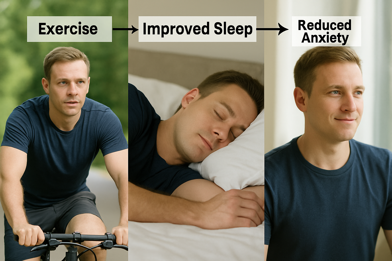
A mediating variable, also known as an intervening variable, helps explain how or why an independent variable (X) influences a dependent variable (Y). It acts as a link in the middle of the cause-and-effect chain, showing the process that connects X to Y. In other words, it tells us what happens in between that helps carry the effect from one variable to the other. Mediating variables are essential for understanding the underlying mechanisms of a relationship, offering insight into the steps or changes that occur between the cause and its outcome. This deeper understanding can improve the accuracy of conclusions drawn from the research and guide more effective interventions. For example, in examining whether exercise reduces anxiety, improved sleep could be a mediating variable. In this case, exercise leads to better sleep, and better sleep then reduces anxiety. Mediators help answer the “how” or “why” behind a causal connection between variables.

Let’s Break it Down- An Example

Show

Mediating Variable

For example, let’s say a study is exploring whether exercise can help reduce anxiety. In this case, improved sleep might be a mediating variable. Exercise may not directly lower anxiety, but it can lead to better sleep, and that improved sleep can then help reduce anxiety. So, better sleep explains how exercise has a calming effect. This illustrates how a mediator helps uncover the underlying process behind the connection, providing a clearer understanding of the relationship between the variables.

*This image was created using ChatGPT; however, the concept, design direction, and creative vision were conceived by Dr. Knight

A moderating variable, or effect modifier, changes the direction or strength of the relationship between an independent and a dependent variable. It acts as a “condition” that influences the degree to which the relationship holds true. In other words, the effect of one variable on another depends on the presence or level of the moderator. The impact of the IV on the DV depends on the level of the moderator.

Let’s Break it down-Example

Show

Moderating Variable

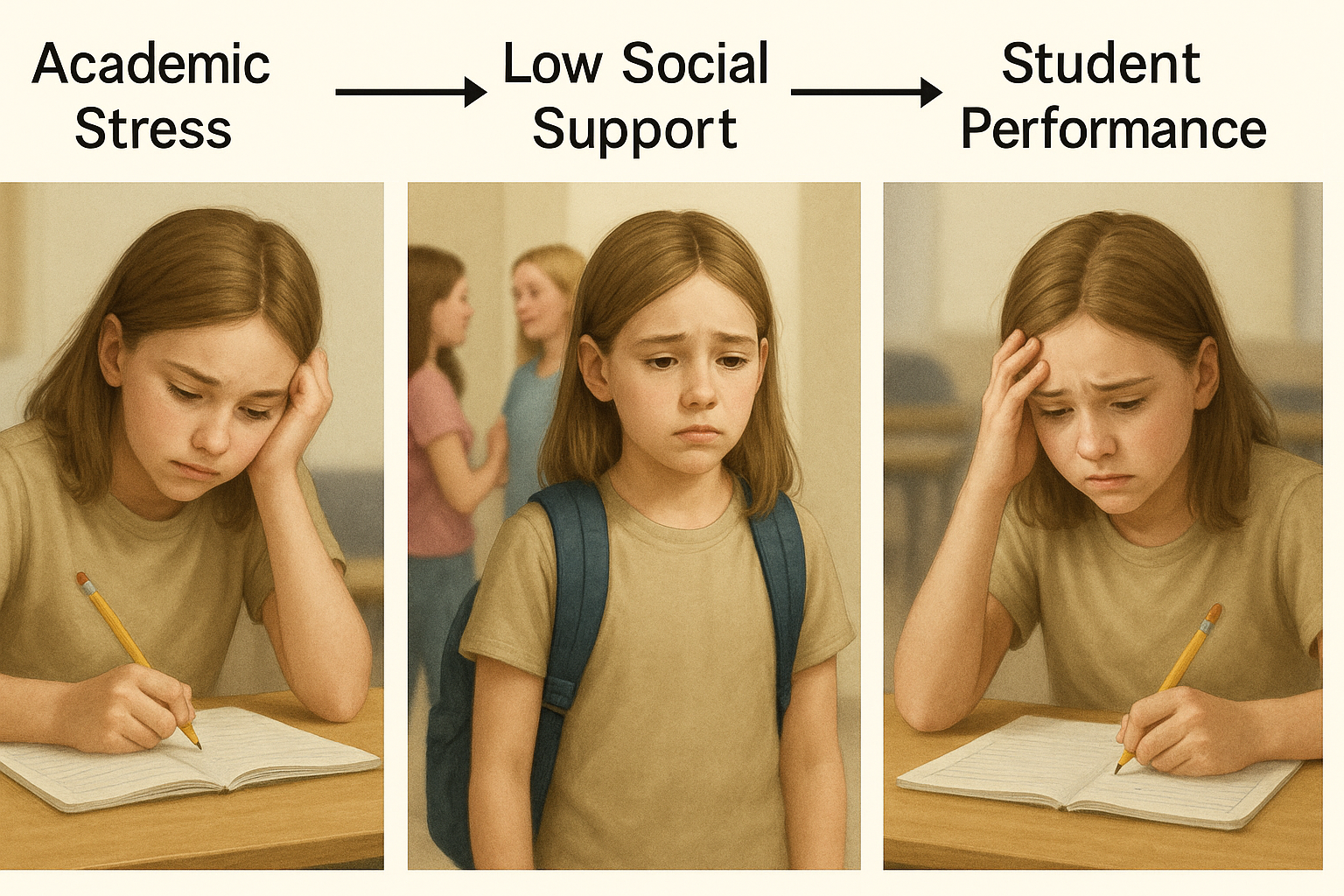
For example, if the independent variable is academic stress, and the dependent variable is student performance, a moderating variable could social support—it could change how much academic stress affects student performance depending on how much social support a student feels.

➤ With High Social Support

Even though the student is experiencing academic stress, having supportive peers helps buffer the negative effects. The student remains emotionally balanced and performs well.

Academic Stress → Social Support → Strong Student Performance

➤ With Low Social Support

The same level of academic stress has a stronger negative effect when the student feels isolated. With little or no support from peers, the student struggles more and performance drops.

Academic Stress → Low Social Support → Struggling Performance]

*These image was created using ChatGPT; however, the concept, design direction, and creative vision were conceived by Dr. Knight


Designing an Experiment

In this section, we look at some different ways to design an experiment. The primary distinction we will make is between approaches in which each participant experiences one level of the independent variable and approaches in which each participant experiences all levels of the independent variable. The former are called between-subjects experiments and the latter are called within-subjects experiments.

Between-Subjects Experiments

In a between-subjects experiment, each participant is tested in only one condition. For example, a researcher with a sample of 100 university students might assign half of them to write about a traumatic event and the other half write about a neutral event. Or a researcher with a sample of 60 people with severe agoraphobia (fear of open spaces) might assign 20 of them to receive each of three different treatments for that disorder. This is the most classic experimental design. It is essential in a between-subjects experiment that the researcher assigns participants to conditions so that the different groups are, on average, highly similar to each other. Those in a trauma condition and a neutral condition, for example, should include a similar proportion of men and women, and they should have similar average intelligence quotients (IQs), similar average levels of motivation, similar average numbers of health problems, and so on. This matching is a matter of controlling these extraneous participant variables across conditions so that they do not become confounding variables.

Random Assignment

The primary way that researchers accomplish this kind of control of extraneous variables across conditions is called random assignment, which means using a random process to decide which participants are tested in which conditions. Do not confuse random assignment with random sampling. Random sampling is a method for selecting a sample from a population, and it is rarely used in psychological research. Random assignment is a method for assigning participants in a sample to the different conditions, and it is an important element of all experimental research. 

In its strictest sense, random assignment should meet two criteria. One is that each participant has an equal chance of being assigned to each condition (e.g., a 50% chance of being assigned to each of two conditions). The second is that each participant is assigned to a condition independently of other participants (meaning we don’t assign two people to the same group because of their association to each other). Thus, one way to assign participants to two conditions would be to flip a coin for each one. If the coin lands heads, the participant is assigned to Condition A, and if it lands tails, the participant is assigned to Condition B. For three conditions, one could use a computer to generate a random integer from 1 to 3 for each participant. If the integer is 1, the participant is assigned to Condition A; if it is 2, the participant is assigned to Condition B; and if it is 3, the participant is assigned to Condition C. In practice, a full sequence of conditions—one for each participant expected to be in the experiment—is usually created ahead of time, and each new participant is assigned to the next condition in the sequence as he or she is tested. When the procedure is computerized, the computer program often handles the random assignment.

One problem with coin flipping and other strict procedures for random assignment is that they are likely to result in unequal sample sizes in the different conditions. Unequal sample sizes are generally not a serious problem, and you should never throw away data you have already collected to achieve equal sample sizes. However, for a fixed number of participants, it is statistically most efficient to divide them into equal-sized groups. It is standard practice, therefore, to use a kind of modified random assignment that keeps the number of participants in each group as similar as possible. One approach is block randomization. In block randomization, all the conditions occur once in the sequence before any of them is repeated. Then they all occur again before any of them is repeated again. Within each of these “blocks,” the conditions occur in a random order. Again, the sequence of conditions is usually generated before any participants are tested, and each new participant is assigned to the next condition in the sequence. Table 5.2 shows such a sequence for assigning nine participants to three conditions. The Research Randomizer website (http://www.randomizer.org) will generate block randomization sequences for any number of participants and conditions. Again, when the procedure is computerized, the computer program often handles the block randomization.

Table 5.2 Block Randomization Sequence for Assigning Nine Participants to Three Conditions
Participant Condition
1 A
2 C
3 B
4 B
5 C
6 A
7 C
8 B
9 A

Random assignment is not guaranteed to control all extraneous variables across conditions. The process is random, so it is always possible that just by chance, the participants in one condition might turn out to be substantially older, less tired, more motivated, or less depressed on average than the participants in another condition. However, there are some reasons that this possibility is not a major concern. One is that random assignment works better than one might expect, especially for large samples. Another is that the inferential statistics that researchers use to decide whether a difference between groups reflects a difference in the population takes the “fallibility” of random assignment into account. Yet another reason is that even if random assignment does result in a confounding variable and therefore produces misleading results, this confound is likely to be detected when the experiment is replicated. The upshot is that random assignment to conditions—although not infallible in terms of controlling extraneous variables—is always considered a strength of a research design.

Matched Groups

An alternative to simple random assignment of participants to conditions is the use of a matched-groups design. Using this design, participants in the various conditions are matched on the dependent variable or on some extraneous variable(s) prior the manipulation of the independent variable. This guarantees that these variables will not be confounded across the experimental conditions. For instance, if we want to determine whether expressive writing affects people’s health then we could start by measuring various health-related variables in our prospective research participants. We could then use that information to rank-order participants according to how healthy or unhealthy they are. Next, the two healthiest participants would be randomly assigned to complete different conditions (one would be randomly assigned to the traumatic experiences writing condition and the other to the neutral writing condition). The next two healthiest participants would then be randomly assigned to complete different conditions, and so on until the two least healthy participants. This method would ensure that participants in the traumatic experiences writing condition are matched to participants in the neutral writing condition with respect to health at the beginning of the study. If at the end of the experiment, a difference in health was detected across the two conditions, then we would know that it is due to the writing manipulation and not to pre-existing differences in health.

Within-Subjects Experiments

In a within-subjects experiment, each participant is tested under all conditions. Consider an experiment on the effect of a defendant’s physical attractiveness on judgments of his guilt. Again, in a between-subjects experiment, one group of participants would be shown an attractive defendant and asked to judge his guilt, and another group of participants would be shown an unattractive defendant and asked to judge his guilt. In a within-subjects experiment, however, the same group of participants would judge the guilt of both an attractive and an unattractive defendant.

The primary advantage of this approach is that it provides maximum control of extraneous participant variables. Participants in all conditions have the same mean IQ, same socioeconomic status, same number of siblings, and so on—because they are the very same people. Within-subjects experiments also make it possible to use statistical procedures that remove the effect of these extraneous participant variables on the dependent variable and therefore make the data less “noisy” and the effect of the independent variable easier to detect. We will look more closely at this idea later in the book.  However, not all experiments can use a within-subjects design, nor would it be desirable to do so.

One disadvantage of within-subjects experiments is that they make it easier for participants to guess the hypothesis. For example, a participant who is asked to judge the guilt of an attractive defendant and then is asked to judge the guilt of an unattractive defendant is likely to guess that the hypothesis is that defendant attractiveness affects judgments of guilt. This knowledge could lead the participant to judge the unattractive defendant more harshly because he thinks this is what he is expected to do. Or it could make participants judge the two defendants similarly in an effort to be “fair.”

Carryover Effects and Counterbalancing

The primary disadvantage of within-subjects designs is that they can result in order effects. An order effect occurs when participants’ responses in the various conditions are affected by the order of conditions to which they were exposed. One type of order effect is a carryover effect. A carryover effect is an effect of being tested in one condition on participants’ behavior in later conditions. One type of carryover effect is a practice effect, where participants perform a task better in later conditions because they have had a chance to practice it. Another type is a fatigue effect, where participants perform a task worse in later conditions because they become tired or bored. Being tested in one condition can also change how participants perceive stimuli or interpret their task in later conditions. This type of effect is called a context effect (or contrast effect). For example, an average-looking defendant might be judged more harshly when participants have just judged an attractive defendant than when they have just judged an unattractive defendant. Within-subjects experiments also make it easier for participants to guess the hypothesis. For example, a participant who is asked to judge the guilt of an attractive defendant and then is asked to judge the guilt of an unattractive defendant is likely to guess that the hypothesis is that defendant attractiveness affects judgments of guilt. 

Carryover effects can be interesting in their own right. (Does the attractiveness of one person depend on the attractiveness of other people that we have seen recently?) But when they are not the focus of the research, carryover effects can be problematic. Imagine, for example, that participants judge the guilt of an attractive defendant and then judge the guilt of an unattractive defendant. If they judge the unattractive defendant more harshly, this might be because of his unattractiveness. But it could be instead that they judge him more harshly because they are becoming bored or tired. In other words, the order of the conditions is a confounding variable. The attractive condition is always the first condition and the unattractive condition the second. Thus, any difference between the conditions in terms of the dependent variable could be caused by the order of the conditions and not the independent variable itself.

There is a solution to the problem of order effects, however, that can be used in many situations. It is counterbalancing, which means testing different participants in different orders. The best method of counterbalancing is complete counterbalancing in which an equal number of participants complete each possible order of conditions. For example, half of the participants would be tested in the attractive defendant condition followed by the unattractive defendant condition, and others half would be tested in the unattractive condition followed by the attractive condition. With three conditions, there would be six different orders (ABC, ACB, BAC, BCA, CAB, and CBA), so some participants would be tested in each of the six orders. With four conditions, there would be 24 different orders; with five conditions there would be 120 possible orders. With counterbalancing, participants are assigned to orders randomly, using the techniques we have already discussed. Thus, random assignment plays an important role in within-subjects designs just as in between-subjects designs. Here, instead of randomly assigning to conditions, they are randomly assigned to different orders of conditions. In fact, it can safely be said that if a study does not involve random assignment in one form or another, it is not an experiment.

A more efficient way of counterbalancing is through a Latin square design which randomizes through having equal rows and columns. For example, if you have four treatments, you must have four versions. Like a Sudoku puzzle, no treatment can repeat in a row or column. For four versions of four treatments, the Latin square design would look like:

A B C D
B C D A
C D A B
D A B C

You can see in the diagram above that the square has been constructed to ensure that each condition appears at each ordinal position (A appears first once, second once, third once, and fourth once) and each condition preceded and follows each other condition one time. A Latin square for an experiment with 6 conditions would by 6 x 6 in dimension, one for an experiment with 8 conditions would be 8 x 8 in dimension, and so on. So while complete counterbalancing of 6 conditions would require 720 orders, a Latin square would only require 6 orders.

Finally, when the number of conditions is large experiments can use random counterbalancing in which the order of the conditions is randomly determined for each participant. Using this technique every possible order of conditions is determined and then one of these orders is randomly selected for each participant. This is not as powerful a technique as complete counterbalancing or partial counterbalancing using a Latin squares design. Use of random counterbalancing will result in more random error, but if order effects are likely to be small and the number of conditions is large, this is an option available to researchers.

There are two ways to think about what counterbalancing accomplishes. One is that it controls the order of conditions so that it is no longer a confounding variable. Instead of the attractive condition always being first and the unattractive condition always being second, the attractive condition comes first for some participants and second for others. Likewise, the unattractive condition comes first for some participants and second for others. Thus any overall difference in the dependent variable between the two conditions cannot have been caused by the order of conditions. A second way to think about what counterbalancing accomplishes is that if there are carryover effects, it makes it possible to detect them. One can analyze the data separately for each order to see whether it had an effect.

Simultaneous Within-Subjects Designs

So far, we have discussed an approach to within-subjects designs in which participants are tested in one condition at a time. There is another approach, however, that is often used when participants make multiple responses in each condition. Imagine, for example, that participants judge the guilt of 10 attractive defendants and 10 unattractive defendants. Instead of having people make judgments about all 10 defendants of one type followed by all 10 defendants of the other type, the researcher could present all 20 defendants in a sequence that mixed the two types. The researcher could then compute each participant’s mean rating for each type of defendant. Or imagine an experiment designed to see whether people with social anxiety disorder remember negative adjectives (e.g., “stupid,” “incompetent”) better than positive ones (e.g., “happy,” “productive”). The researcher could have participants study a single list that includes both kinds of words and then have them try to recall as many words as possible. The researcher could then count the number of each type of word that was recalled. 

Between-Subjects or Within-Subjects?

Almost every experiment can be conducted using either a between-subjects design or a within-subjects design. This possibility means that researchers must choose between the two approaches based on their relative merits for the particular situation.

Between-subjects experiments have the advantage of being conceptually simpler and requiring less testing time per participant. They also avoid carryover effects without the need for counterbalancing. Within-subjects experiments have the advantage of controlling extraneous participant variables, which generally reduces noise in the data and makes it easier to detect a relationship between the independent and dependent variables.

A good rule of thumb, then, is that if it is possible to conduct a within-subjects experiment (with proper counterbalancing) in the time that is available per participant—and you have no serious concerns about carryover effects—this design is probably the best option. If a within-subjects design would be difficult or impossible to carry out, then you should consider a between-subjects design instead. For example, if you were testing participants in a doctor’s waiting room or shoppers in line at a grocery store, you might not have enough time to test each participant in all conditions and therefore would opt for a between-subjects design. Or imagine you were trying to reduce people’s level of prejudice by having them interact with someone of another race. A within-subjects design with counterbalancing would require testing some participants in the treatment condition first and then in a control condition. But if the treatment works and reduces people’s level of prejudice, then they would no longer be suitable for testing in the control condition. This difficulty is true for many designs that involve a treatment meant to produce long-term change in participants’ behavior (e.g., studies testing the effectiveness of psychotherapy). Clearly, a between-subjects design would be necessary here.

Remember also that using one type of design does not preclude using the other type in a different study. There is no reason that a researcher could not use both a between-subjects design and a within-subjects design to answer the same research question. In fact, professional researchers often take exactly this type of mixed methods approach.

References

  1. McCoy, S. K., & Major, B. (2003). Group identification moderates emotional response to perceived prejudice. Personality and Social Psychology Bulletin, 29, 1005–1017. 
  2. Babbie, E. (2010). The practice of social research (12th ed.). Wadsworth
  3. Campbell, D., & Stanley, J. (1963). Experimental and quasi-experimental designs for research. Rand McNally. 
  4. Pepin, J. R. (2019). Beliefs About money in families: Balancing unity, autonomy, and gender equality.Journal of Marriage and Family, 81(2), 361-379. https://doi.org/10.1111/jomf.12554


License

Icon for the Creative Commons Attribution-ShareAlike 4.0 International License

Understanding Research Design in the Social Science Copyright © by Utah Valley University is licensed under a Creative Commons Attribution-ShareAlike 4.0 International License, except where otherwise noted.

Share This Book