Data Preparation and Descriptive Statistics
Goal of Analysis
“Analyze and evaluate data” is the fourth step in the research process. During this step, our goal is to make sense of all the beautiful data that were generated in our study! We spent all that time designing a good study, so now we get the opportunity to reap our rewards and learn what the data can tell us. Because this texts’ focus is on research design, and there are entire other textbooks and classes on analysis, we’ll only scratch the surface of analysis concerns here. If you’re interested in actually doing some research or seeing more details of how to treat the data, then you would do well to take some statistics courses or qualitative data analysis courses, depending on what data you’re thinking about!
Whether your data are words, numbers, videos, or some other type, the first step to analysis is actually preparation. The data are rarely usable directly out of a study, and careful preparation is important to making sure our analyses are correct. Thus, let’s talk about “cleaning” quantitative data and preparing them for analysis.
Building a codebook
One of the key goals of quantitative analysis is to condense the data into manageable, analyzable bits; having 100 completed questionnaires is great, but if each questionnaire has 50 questions, you have a lot of data coming your way. While this may sound daunting, one major advantage of quantitative methods such as surveys and experiments is that they enable researchers to describe large amounts of data because they can be represented by and condensed into categories and numbers.
To condense your completed surveys into analyzable numbers, you’ll first need to create a codebook. A codebook is a document that outlines how a researcher has translated their data from words (or other data, like behavioral observations) into numbers. An excerpt from a codebook can be seen below. As you’ll see in the table, in addition to converting response options into numerical values, a short variable name is given to each question. This shortened name comes in handy when entering data into a computer program for analysis.
| Variable # | Variable Name | Question | Options |
| 11 | FINSEC | In general, how financially secure would you say you are? | 1 = Not at all secure |
| 2 = Between not at all and moderately secure | |||
| 3 = Moderately secure | |||
| 4 = Between moderately secure and very secure | |||
| 5 = Very secure | |||
| 12 | FINFAM | Since age 62, have you ever received money from family members or friends to help make ends meet? | 0 = No |
| 1 = Yes | |||
| 13 | FINFAMT | If yes, how many times? | 1 = 1 or 2 times |
| 2 = 3 or 4 times | |||
| 3 = 5 times or more | |||
| 14 | FINCHUR | Since age 62, have you ever received money from a church or other organization to help make ends meet? | 0 = No |
| 1 = Yes | |||
| 15 | FINCHURT | If yes, how many times? | 1 = 1 or 2 times |
| 2 = 3 or 4 times | |||
| 3 = 5 times or more | |||
| 16 | FINGVCH | Since age 62, have you ever donated money to a church or other organization? | 0 = No |
| 1 = Yes | |||
| 17 | FINGVFAM | Since age 62, have you ever given money to a family member or friend to help them make ends meet? | 0 = No |
| 1 = Yes |
The next task after creating your codebook is data entry. If you’ve utilized an online tool such as SurveyMonkey or Qualtrics to administer your questionnaire, here’s some good news: Most online survey tools can import survey results directly into a data analysis program. This is excellent news; not only does it save time, but it also reduces the risk of entry errors that are a risk of manual data entry – either on the side of those entering the data (mistyping a number) and those that come from participants (is that a 4 or a 2 that someone wrote? Handwriting is not always easy to read!). If errors are made in data entry, it can jeopardize the results of the project, so if manual entry is required, each entry should be double-checked (a process called validation or double entry). Any errors that are true errors in data entry need to be corrected (one person typed in a 2 instead of 3 when entering data from a paper survey, for example), but if it’s just a weird data point, an outlier, it should not be changed, just noted. If manual entry can be avoided, even better, though it is still important to review the data for weird qualities (which is why we calculate descriptive statistics first).
Coding Quantitative Data
Getting all the data into numeric form is often one of the most boring parts of the research process, depending on the method that was used to collect the data. If you’re coding the data in a quantitative fashion, you’re assigning numbers. Coding may be fairly straightforward if your variable is already numeric, such as with a variable like height: you can just record the inches or centimeters of the person’s height (but you must decide which one first, and note the decision in your codebook!). You may have to assign numbers, though, to something that isn’t inherently numeric, like a Likert scale (this is ordinal data, so the numbers only tell us order):
1 = very unhappy, 2 = somewhat unhappy, 3 = neither happy or unhappy, 4 = somewhat happy, 5 = very happy.
or a nominal (so order isn’t even at play) variable like eye color:
1 = brown, 2 = blue, 3 = green, 4 = hazel, 5 = gray
As you’re making these assignments, you should be building the codebook to record the choices you made – is height recorded as inches or centimeters? Does 1 = very unhappy or very happy? Which numbers are which hair color?
Suppose you have some observational data that you’ve recorded in video or audio. Coding that data also means assigning numbers if you want to do statistics on it. Often, you’ll want at least two people to act as coders so that you can assess their similarity as a form of reliability (inter-rater reliability to be specific). Having clear guidelines (usually in a coding protocol) regarding what is scored and how is important; that’s really beyond or scope in this book, but if quantitative observations are of interest to you, seek out additional experience (many researchers who do this kind of research will pay undergraduates to do the coding part!) or classes on this topic.
However you do it, the goal in quantitative analysis is to make everything numeric. The most basic way to enter data into a spreadsheet is to make one row equal one person or observation in your data (called wide format). You’ll end up with a header row (with the name of the variables) and then n rows after that, with n = sample size for your study, like the image below, which is the first nine rows and five variables of an imaginary dataset:

The codebook for these data might look something like this:
_____________________________________
id: id of participant assigned at first interview. 1-9
marstat: marital status of participant, reported at first interview. 1 = single, 2 = married, 3 = divorced, 4 = widowed
educ: years of education completed, reported at first interview. 12 = high school, 14 = AS or AA degree, 16 = BS or BA degree, 20 = PhD
happy1: self-report of happiness, first interview. 1 = very unhappy, 2 = somewhat unhappy, 3 = neither happy or unhappy, 4 = somewhat happy, 5 = very happy.
happy2: self-report of happiness, second interview. 1 = very unhappy, 2 = somewhat unhappy, 3 = neither happy or unhappy, 4 = somewhat happy, 5 = very happy.
_____________________________________
Cleaning & Final Preparation
After we’ve entered everything, we may then need to do some data manipulation. Although you might think of the word “manipulation” as a bad thing, in this case we’re not talking about the unethical kind where we change the information! Rather, in this case, manipulation refers to some basic mathematical operations that allow us to make the data more usable, such as generating the summary scores from scales (the “overall score” for a scale with multiple questions), reverse code variables that were presented in opposite order (sometimes a scale with multiple questions will present some of the questions with negative wording to check that respondents are paying attention), and sometimes transform data into a useful form (like instead of reporting income in dollars, we collapse it into five meaningful categories based on the values in our sample). This is also when we assess the patterns of missing data (cases where someone didn’t answer a question, for example, or errors where some folks weren’t presented with all questions) present in our dataset and choose how to deal with it.
Once are data are in the spreadsheet, documented, clean, and in a useful form, we’re ready to start looking for patterns!
Identifying patterns
Descriptive statistics are immensely important for understanding what our data tell us. The name of this group of statistics refers to what it sounds like: the characteristics of quantitative data that describe what’s going on. This is in contrast to inferential statistics, which is what we do when we are seeking to test statistical hypotheses. If you’ve read a research article that talked about t-tests, z-tests, p-values, or regression coefficients (or hundreds of other weirdly-named statistics) you’ve seen the results of inferential statistics. They are important and helpful, but mostly beyond the scope of this book. Descriptives statistics are immensely important, and even if your goal is to eventually run inferential statistics, one must have a solid basis of description in their dataset to understand what inferences can be made. in some cases, descriptive statistics are actually the goal in and of themselves! Descriptive statistics can tell us everything from the central tendency of a variable to its variance and distribution, to its correlation to something else, and lots of other things.
Data analysis is about identifying, describing, and explaining patterns. Univariate analysis is the most basic form of analysis that quantitative researchers conduct. In this form, researchers describe patterns across just one variable (hence the “uni” part of the name). Univariate analysis includes frequency distributions and measures of central tendency. A frequency distribution is a way of summarizing the distribution of responses on a single survey question. Let’s look at the frequency distribution for just one variable from a survey of older workers. We’ll analyze the item mentioned first in the first codebook excerpt given earlier, which is on respondents’ self-reported financial security.
| In general, how financially secure would you say you are? | Value | Frequency | Percentage |
| Not at all secure | 1 | 46 | 25.6 |
| Between not at all and moderately secure | 2 | 43 | 23.9 |
| Moderately secure | 3 | 76 | 42.2 |
| Between moderately and very secure | 4 | 11 | 6.1 |
| Very secure | 5 | 4 | 2.2 |
| Total valid cases = 180; no response = 3 |
As you can see in the frequency distribution on self-reported financial security, more respondents reported feeling “moderately secure” than any other response category. We also learn from this single frequency distribution that fewer than 10% of respondents reported being in one of the two most secure categories.
Another form of univariate analysis that survey researchers can conduct on single variables is measures of central tendency. Measures of central tendency can be taken for variables at any level of measurement, from nominal to ratio, but the correct statistic must be used for each level of measurement. There are three measures of central tendency: modes, medians, and means. Mode refers to the most common response given to a question. Modes are most appropriate for nominal-level variables. A median is the middle point in a distribution of responses; this obviously requires that order be present in the variable. Finally, the measure of central tendency used most often for interval- and ratio-level variables is the mean. More commonly known as an average, means can be obtained by adding the value of all responses on a given variable and then dividing that number of the total number of responses.
Median is the appropriate measure of central tendency for ordinal-level variables, though it is sometimes used for interval or ratio variables whose distribution contains outliers or extreme scores that would skew the mean higher than the true center of the distribution. For example, if you asked your four friends about how much money they have in their wallets and one of them just won the lottery, the mean would be quite high, even though most of you do not have near that amount. In that case, the median value would be closer to the true center than the mean.
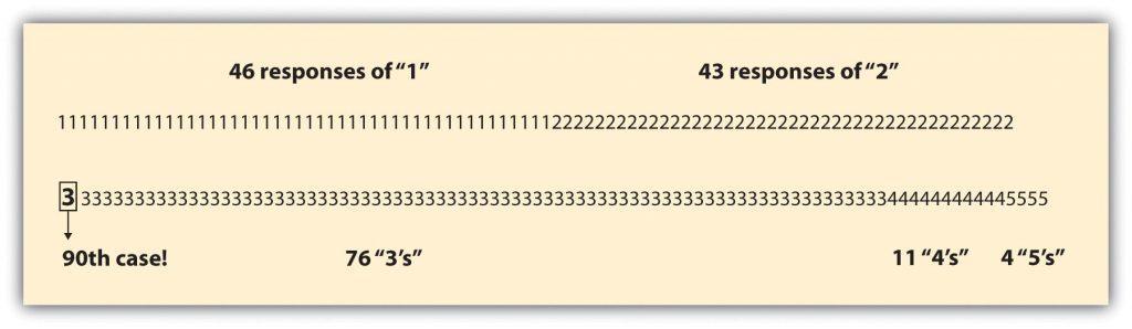
In the previous example of older workers’ self-reported levels of financial security, the appropriate measure of central tendency would be the median, as this is an ordinal-level variable. If we were to list all responses to the financial security question in order and then choose the middle point in that list, we’d have our median. In the figure below, the value of each response to the financial security question is noted, and the middle point within that range of responses is highlighted. To find the middle point, we simply divide the number of valid cases by two. The number of valid cases, 180, divided by 2 is 90, so we’re looking for the 90th value on our distribution to discover the median. As you’ll see below, that value is 3; thus, the median on our financial security question is 3 or “moderately secure.”
As you can see, we can learn a lot about our respondents simply by conducting univariate analysis of measures on our survey. We can learn even more, of course, when we begin to examine relationships across multiple variables. This latter type of analysis is known as multivariate analysis.
Bivariate analysis allows us to assess covariation among two variables. This means we can find out whether changes in one variable occur together with changes in another (not trying to prove if one causes the other, just looking at how they vary together). If two variables do not covary, they are said to have independence, which simply means that there is no relationship between the two variables in question. To learn whether a relationship exists between two variables, a researcher may cross-tabulate the two variables and present their relationship in a contingency table. A contingency table shows how variation on one variable may be contingent on variation on the other.
Let’s look at a contingency table to get a visual representation. In the table below, we have a cross-tabulation of two questions from an older worker survey: respondents’ reported gender and their self-rated financial security.
| Men | Women | |
| Not financially secure (%) | 44.1 | 51.8 |
| Moderately financially secure (%) | 48.9 | 39.2 |
| Financially secure (%) | 7.0 | 9.0 |
| Total | N = 43 | N = 135 |
In the table, you’ll notice that we collapsed a few of the financial security response categories (recall there were five categories presented in the earlier table). Sometimes researchers will collapse response categories on similar items to make the results easier to read. You’ll also see that we placed the variable “gender” in the table’s columns and “financial security” in its rows. Typically, values that are contingent on other values (dependent variables) are placed in rows, while independent variables are placed in columns. This simplifies the comparison across categories of our independent variable.
Reading across the top row of our table, we can see that around 44% of men in the sample reported that they are not financially secure while almost 52% of women reported the same. In other words, more women than men reported they are not financially secure. You’ll also see in the table that we reported the total number of respondents for each category of the independent variable in the table’s bottom row. This is also standard practice in a bivariate table, as is including a table heading describing what is presented in the table.
Researchers interested in simultaneously analyzing relationships among more than two variables conduct multivariate analysis. If we hypothesized that financial security declines for women as they age but increases for men as they age, we might consider adding age to the preceding analysis. To do so would require multivariate, rather than bivariate, analysis. This is common in studies with multiple independent or dependent variables. It is also necessary for studies that include control variables, which almost all studies do. We won’t go into detail about how to conduct multivariate analysis of quantitative survey items here, as that’s getting into the inferential realm of statistics. If you are interested in learning more about the analysis of quantitative survey data, check out your campus’s offerings in statistics classes. The quantitative data analysis skills you will gain in a statistics class could serve you quite well should you find yourself seeking employment one day.
Image Attribution
Figure showing median value copied from Blackstone, A. (2012). Principles of sociological inquiry: Qualitative and quantitative methods. Saylor Foundation. Retrieved from: https://saylordotorg.github.io/text_principles-of-sociological-inquiry-qualitative-and-quantitative-methods/ Shared under CC-BY-NC-SA 3.0 License (https://creativecommons.org/licenses/by-nc-sa/3.0/
