We’ve talked about “correlational designs” in the past, but correlation is also a statistic. Specifically, the correlation coefficient, represented by r, is a measure of how much two variables are related to each other. It bears repeating that correlation does not tell us causation; x and y being correlated does not require that either one causes the other. In fact, there are some ridiculous spurious (non-causal) correlations out there if you start comparing random trends to each other. If you want to see some examples, play around with this website dedicated to them (though please be aware that death rates apparently correlate with a lot of things, so there are some morbid charts in this site): Spurious Correlations.
Interpreting Correlations
A correlation coefficient, often represented with r, can only range from -1 to 1. If r = 0, then there is no relationship between the two variables under study. As r approaches either -1 or 1 (absolute 1, or |1|), the relationship is indicated to be stronger and stronger. At either value of |1|, the relationship is perfect, such that a change of 1 in X is always accompanied by a change of 1 in Y. The sign of the correlation (- or +) does not have anything to do with how strong the relationship is. Rather, the sign indicates the direction of the relationship: positive (as one variable goes up, the other one does too) or negative (as one goes up, the other goes down). Thus, r = -.84 is a stronger relationship than r = .25, but one is negative and the other is positive.
What does that look like graphically?
If you drew a straight line through the points on the scatter plot, which we talked about in the last section, the direction of the line (up or down as it moved left to right) would tell you the direction; up is positive, down is negative. The closer the points cluster to the line indicates the strength of the relationship; if they’re right on the line or very close, the relationship is stronger than if the point are spread out and the pattern is less clear.
See the graphs below for examples:
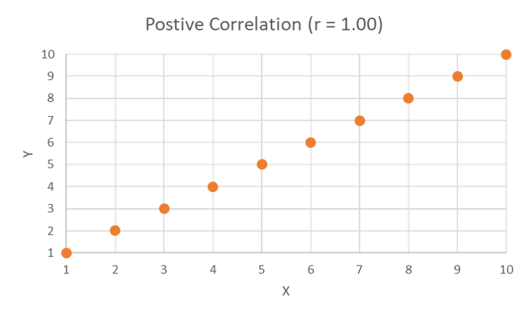
This scatter plot shows a positive correlation of 1, in that all points on the graph fall perfectly on a line that moves from the lower-left corner to the upper-right corner.
https://uen.pressbooks.pub/app/uploads/sites/524/2025/06/pos92.png
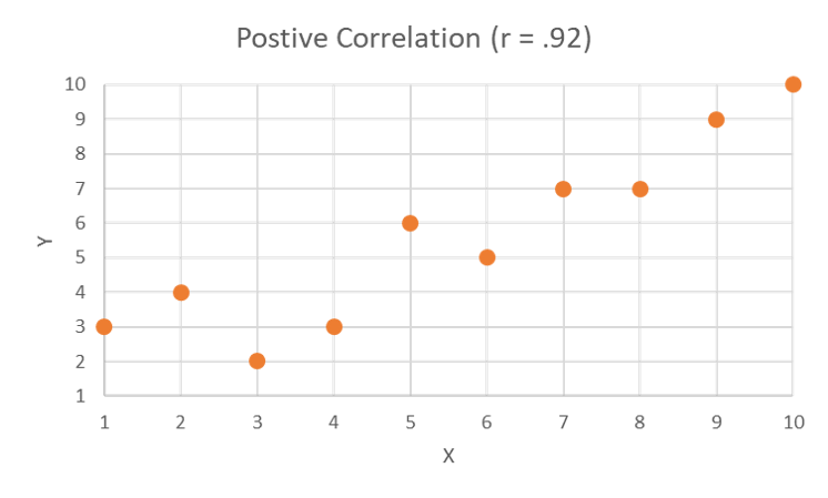
This scatterplot shows a strong, but not perfect, positive correlation. The points cluster tightly around a line extending from bottom left to upper right.
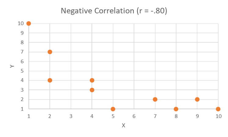
This scatterplot shows a strong, but not perfect, negative correlation. The points cluster around a line extending from upper left to lower right.
All of these are fairly strong; once you move down to a weaker correlation, it can be harder and harder to visually see the pattern. That’s why the actual statistic is helpful; that little r value tells you a lot in a tiny bit of space, so be sure to read those when you see them.
Linear regression is an extension of correlation whereby values of one variable (Y) are predicted by values of the other variable (X) when both variables are ratio or interval. There are other types of regressions used for ordinal and nominal data or combinations (you may have seen “logistic” tossed around, for example). Regressions can get very complicated very quickly (control variables usually come into play too, something we talked about back in the chapter on quantitative data collection), but it’s important to recognize that, at the core, they’re just correlations.
Inferential Statistics
Don’t over-interpret descriptive statistics! Descriptive statistics tell us a lot; the distribution, central tendency, variability, and correlations in a study are sometimes all we really want to know. When we want to start making comparisons and testing hypotheses, though, we need to look to another class of statistics: inferential statistics. If we wanted to, for example, we could make and test some hypotheses about the population of Utah from a hypothetical survey I could take of ice-cream eaters across the state. We’d have to start testing things statistically, however, to truly understand if our data support our hypotheses or not.
What if we hypothesized that people who prefer chocolate ice cream are older than people who prefer vanilla ice cream? We could calculate the values within the sample separately and compare them on a bar graph, but what could we conclude from this? Without applying inferential statistics, we can say that it appears chocolate lovers are older than vanilla fans by about 3 years on average, let’s say, but we don’t know if that’s statistically different, meaning there’s a chance (and we don’t know what that chance is until we apply some inferential statistics) that the difference we’re observing here is completely due to randomness in the sample selection – maybe we randomly found the oldest chocolate lovers in Utah – so we can’t speak conclusively on this. If we were to apply a test (likely a t-test in this case, for those who have taken a stats class), we could generate a probability statistic to help decide if this is “statistically significant” or not. Even if we don’t, however, the descriptive statistics from this sample still give us some data to work with and interesting information about the sample.
This is all this to say: be careful not to over-interpret things. Sometimes descriptives are enough, and if they are, then use them to their fullest and don’t push them. If you need to go further and test things, make sure you’re being careful; there are whole classes (and honestly, whole degrees and careers, if you really want to get into it) dedicated to understanding inferential stats, so it’d be recommended you take one of those or find someone to work with who knows what they’re doing if you need that.
