9 Example 2-6 Bounce Diagram (Step Function & Pulse)

APP THUMBNAIL

IN TEXT DESCRIPTION;

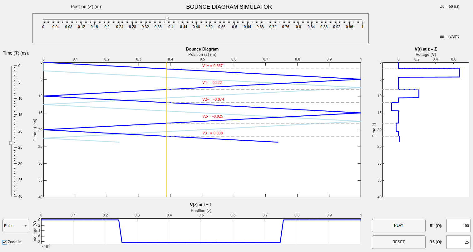
Below is the bounce diagram application. To properly visualize the evolution of a pulse across a 1-meter transmission line, a voltage versus time graph is provided to the right of the bounce diagram, and a voltage versus position graph is provided below the bounce diagram. These supplementary graphs are aligned with the time and position axes of the bounce diagram so you can track how the wavefront affects the evolution of the voltage on the transmission line. You may examine the voltage versus time at a particular point on the transmission line by using the position slider at the top. The yellow vertical line marks that position. To more easily track how the wavefront changes the voltage at that point “Z”, dashed lines are provided on the bounce diagram and voltage versus time graph. You may also examine the transmission line at a particular time “T” by using the slider on the left. The slider will automatically run if you use the “Play” button in the bottom right corner. Reflected values will automatically appear along the bounce diagram. You may also select between a step function or a 2.5 ns pulse indicated on the bottom left. Finally, a “zoom” feature will allow you to better see the pulse or step signal shape on the voltage versus position graph on the bottom.

APP LINK

https://matlab.mathworks.com/open/github/v1?repo=cfurse/ElectromagneticsTextbookCode&file=Applications/BounceDiagramSimulation.mlapp&focus=true

bounce diagram app

Ω

VIDEOS:

To explore more different scenarios, see the bounce diagram app.

IN TEXT DESCRIPTION (RS 25 || RL 50 || PULSE)

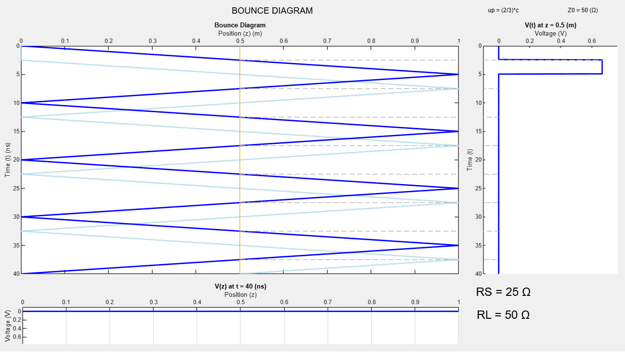
In this video, the load is matched with the transmission line, so all of the energy is transferred to the load and nothing is reflected. You’ll see the voltage spike at the halfway point on the transmission line on the voltage versus time graph and remain at zero afterward. The initial pulse on the voltage versus position graph will travel rightward but not be reflected.

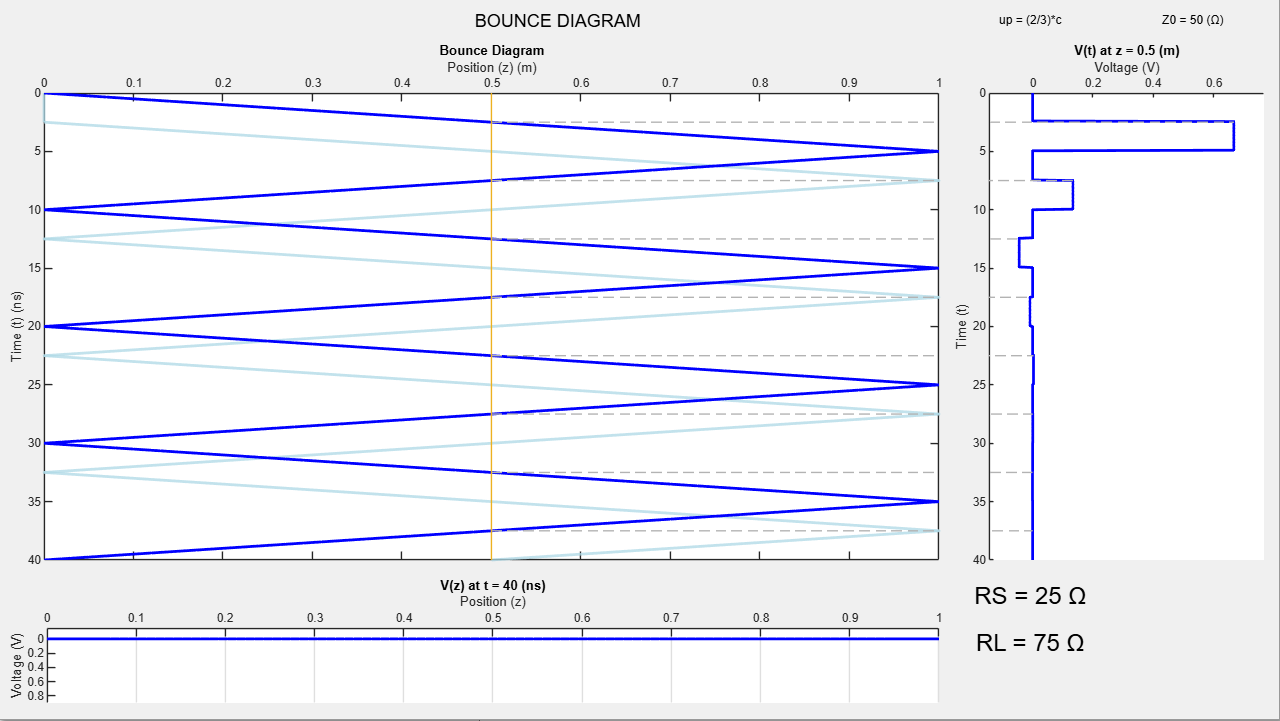
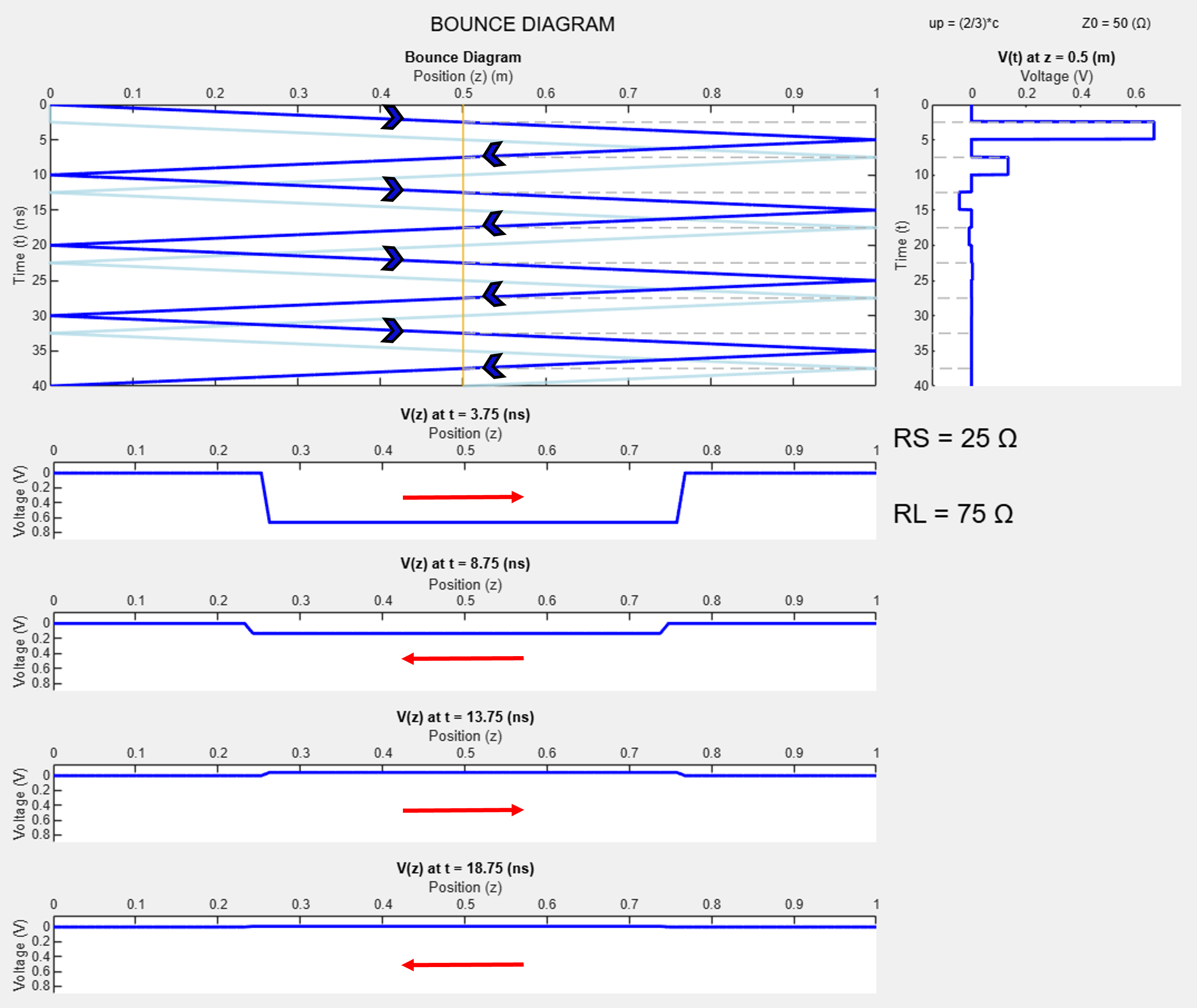
IN TEXT DESCRIPTION (RS 25 || RL 75 || PULSE)

In this video, the 75 Ω load is not matched with the transmission line. Remember that when analyzing a pulse on a bounce diagram, you can break the signal down into a 1 V voltage source step function and a delayed -1 V voltage source step function to understand the voltage versus time graph. Here, we are looking at the halfway point on the transmission line. (TODO add equation?) First, the 1 V voltage source is transferred onto the line as 0.67 V and passes through the halfway point at 2.5 ns. 2.5 ns later, the -1 V voltage source is transferred onto the line as -0.67 V. This yields a 0 V signal at the halfway point at 5 ns  seen on the voltage versus time graph. The reflection coefficient at the load in this scenario is 0.2, so only some of the voltage is reflected back for our 0.67 V signal. You can see this at 7.5 ns when a .2*.67 = .134 V signal passes through the halfway point. The -1 V voltage source signal follows behind at -.134 V and cancels it out, resulting in yet again 0 V. Since the pulse is short enough in duration for our designated location, it will be easy to see the pulse shape on the voltage versus time graph.

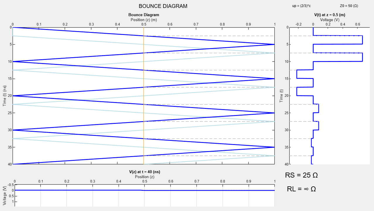
IN TEXT DESCRIPTION: (RS 25 || RL inf || PULSE)

In the below scenario, we have an open load and therefore a complete 1 reflection coefficient. You’ll notice that the entire pulse signal is reflected at the load but the 25 Ω source impedance will dissipate the signal over time. This results in a unique pattern where you see the same pulse voltage repeat itself once before changing magnitude. First you’ll see two 0.67 V pulses, followed by two -0.22 V pulses after that and so on.

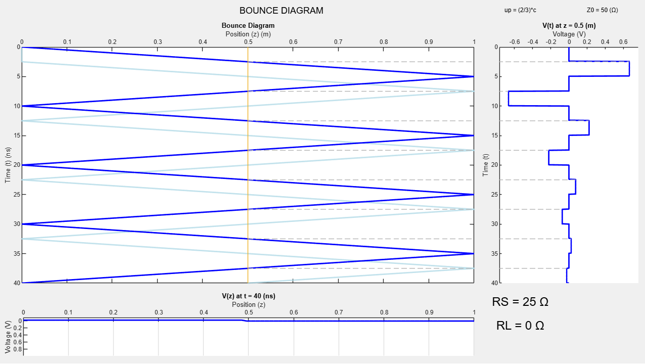
IN TEXT DESCRIPTION (RS 25 || RL SHORT || PULSE)

In this scenario, the load is a short, resulting in a complete -1 reflection coefficient. Similar to the scenario above, you’ll see the same value repeat its negative self before the 25 Ω source impedance changes the magnitude of the traveling pulse. At the start, a 0.67 V signal will pass through the center of the transmission line. Shortly after, a -0.67 V signal will pass through. The source will then reflect the signal at 0.22 V. The pattern continues.

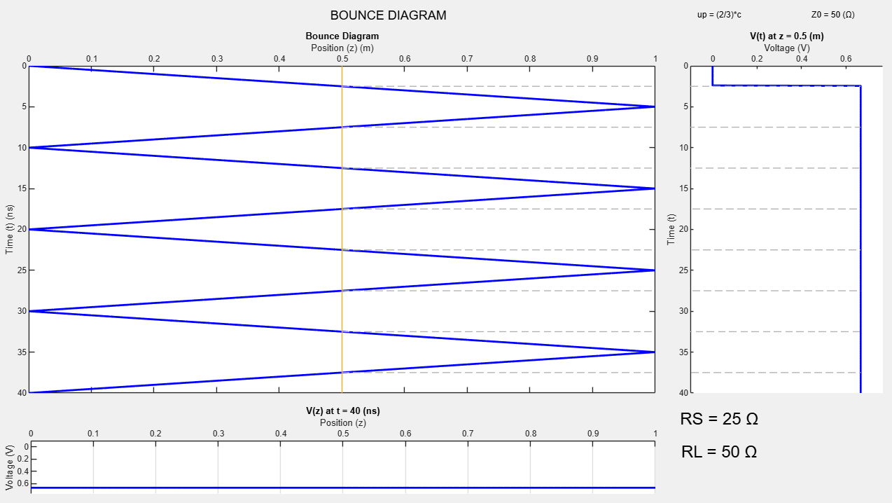
In the following scenarios, a 1 V signal is sent down the 50 Ω transmission line in the form of a step function.

IN TEXT DESCRIPTION (RS 25 || RL MATCH || STEP)

In this scenario, the 50 Ω load is matched with the transmission line, so there aren’t any reflections. The 1 V signal simply goes onto the transmission line as 0.67 V and is absorbed by the load entirely.

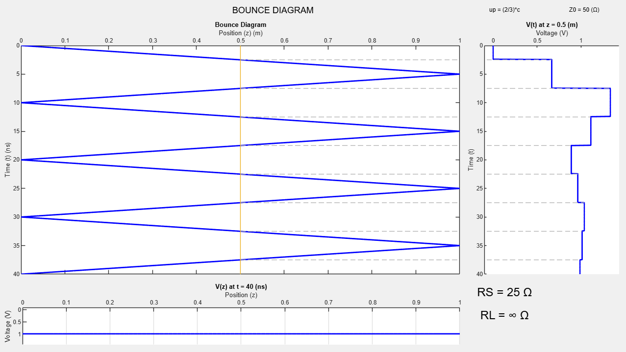
IN TEXT DESCRIPTION (RS 25 || RL OPEN|| PULSE)

Below, the complete 1 reflection coefficient means that the center of our transmission line will momentarily rise above the 1 V signal. First, a 0.67 V signal passes through and then a 0.67 V signal is reflected back, resulting in a 1.33 V signal. Again, the source impedance will dissipate the signal until it stabilizes at the desired 1 V. However, this momentary increase is important to keep in mind especially at higher voltages.

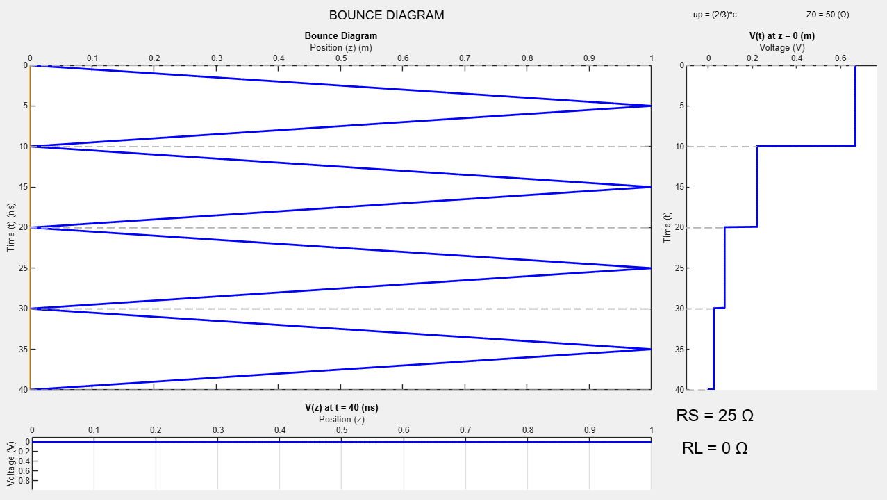
IN TEXT DESCRIPTION (RS 25 || RL SHORT || STEP || AT SOURCE)

Below, the load is a short, resulting in a complete -1 reflection coefficient. Notice that the voltage versus time graph will evaluate the voltage at the source instead of the center of the transmission line like many of the other figures and videos. The signal slowly decreases over time as the source dissipates the signal. (TODO add?)

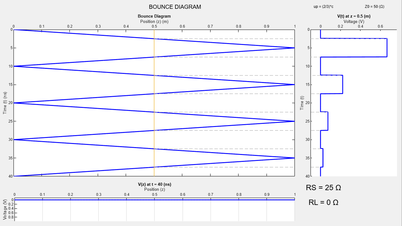
IN TEXT DESCRIPTION (RS 25 || RL SHORT || STEP || AT CENTER)

This is the exact same scenario as above, however the point of interest is now the center of the transmission line. Notice that since the reflection coefficient is -1, the center of the transmission line will reach 0 periodically before the source’s reflection will change its value. First, 0.67 V passes through. Next, the V1- signal of -0.67 V passes through and the total voltage at the center is 0 V. The V1- signal reaches the source and is reflected as 0.22 V and the cycle continues.

STILL

IN TEXT DESCRIPTION:

SCREEN READER DESCRIPTION:

IN TEXT DESCRIPTION:

TODO

SCREEN READER DESCRIPTION: