Graded Potentials and Summation
Objective 10
Define graded potentials. Compare and contrast graded potentials and action potentials. Illustrate the concepts of temporal and spatial summation.
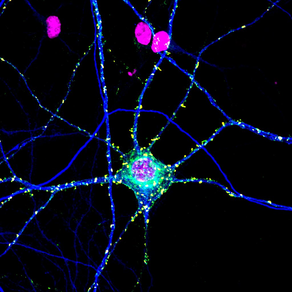
This picture shows a specially stained neuron. The DNA is in magenta; you can see the nucleus inside the cell body and also three glial cell nuclei nearby. The light and dark blue staining is part of the neuron’s cytoskeleton. Axons are stained dark blue in this fluorescence photomicrograph because they are rich in microtubules. Synaptic terminals are stained yellow.
The “average” neuron receives 10,000 inputs from other neurons. (It then follows that the “average” neuron sends 10,000 outputs via presynaptic terminals to other neurons.)
The overarching question in this objective, then, is what the neuron does with those 10,000 inputs. How does the geometry of the neuron relate to processing?
The secret is graded potentials. We’ve already learned about the action potential. (Remember that potential = voltage.)
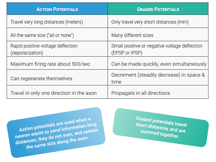
Action potentials are used when a neuron wants to send information long distances; they do not sum, and remain the same size along the axon.
Graded potentials travel short distances and are summed together.
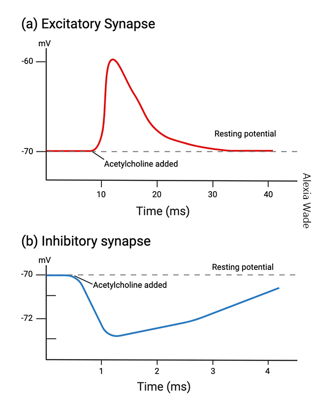
Graded potentials typically (though not always) arise in the postsynaptic membrane due to the action of ligand-gated ion channels. For example, if a ligand binds to a ligand-gated channel, that channel opens, and allows Na+ to enter the neuron across the postsynaptic membrane, then the positively charged sodium ions entering the postsynaptic neuron cause it to depolarize (become more positive). If a ligand binds to a channel, that channel opens, and allows K+ to exit the neuron across the postsynaptic neuron, then the positively charged potassium ions leaving the postsynaptic neuron cause it to hyperpolarize (become more negative).
The effect of the neurotransmitter acetylcholine is a good example of both these effects. Nicotinic acetylcholine receptors cause depolarization of the neuron; muscarinic acetylcholine receptors cause hyperpolarization of the neuron.
Amazingly, scientists have measured the flow of ions through an individual nicotinic ACh receptor using a technique called patch clamping. The current (flow of ions over time) is about 2 billionths of an ampere (2 pA). This represents the flow of roughly 10,000 ions. A typical synapse might have 300,000 such channels representing the flow of 3,000,000,000 sodium ions. This would correspond to a potential change of about 30 mV, or about 100 million ions per mV change. These numbers are not to learn, but merely for you to place in your personal Gee Whiz Biology File. (Thanks, Dr. Beth Burnside, for creating my Gee Whiz Biology File that I pulled this out of!)
The muscarinic acetylcholine receptor is a G protein-coupled receptor which activates a signal-gated potassium channel. Potassium leaves the neuron, resulting in hyperpolarization. See it illustrated on 13-64, Obj. 12.
Graded potentials, as the name implies, are all different sizes. Typically, they are no more than a few millivolts in size. (Remember a “typical” action potential is about 100 mV in amplitude.)
Graded potentials can either represent a negative deflection in membrane voltage or a positive deflection in membrane voltage.
There are two possible modes of output for the neuron. Neurons which send information over a long distance fire action potentials starting at the initial segment; when the action potential reaches the axon terminals, it triggers the release of neurotransmitter.
Neurons which only carry information a short distance have a different strategy. In those neurons, synaptic release is triggered directly by a voltage change at the synapse large enough to bring voltage-gated Ca2+ channels to threshold. We will see how we get that in a later part of this objective.
The negative deflection in voltage pulls the neuron away from the threshold for doing something. Because it makes synaptic release or an action potential less likely, it is called an inhibitory postsynaptic potential (IPSP).
The positive deflection in voltage brings the neuron closer to the threshold for doing something. Because it makes synaptic release or an action potential more likely, it is called an excitatory postsynaptic potential (EPSP).
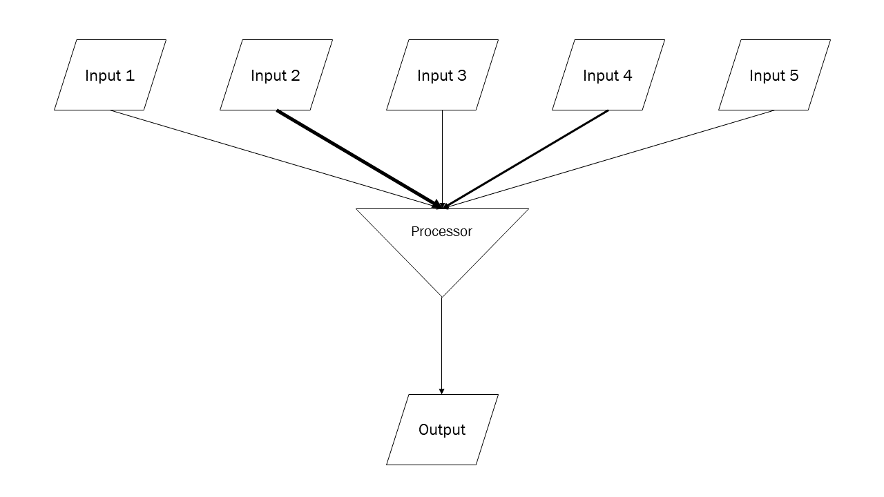
Please don’t make fun of my homemade diagram, but I couldn’t find one that showed what I wanted to show so I made one of my own. Those with computer programming experience will understand how I’ve represented inputs and outputs with parallelograms and a processor with an inverted triangle. The neuron receives about 10,000 synaptic inputs, but only 5 are shown here. Each of those 5 inputs has a different inherent strength (represented by the weight of the arrow connecting the input to the processor). The processor adds all those inputs together and decides: should I create an output? If yes, then the output (action potential or synaptic release) occurs; if no, then it doesn’t.
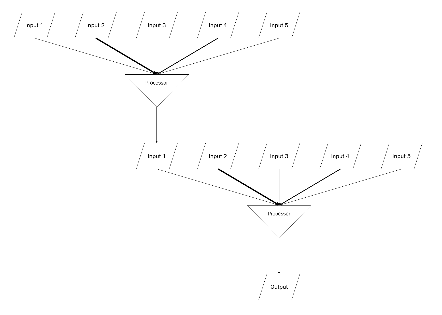
Now imagine one of these groups of 5 synapses is on a small, distant branch of the dendritic tree, and another 5 are on another small, distant branch, and so forth.
Each branch point of the dendritic tree would represent a sort of processor, where voltage changes would be brought together, compiled, and an output generated.
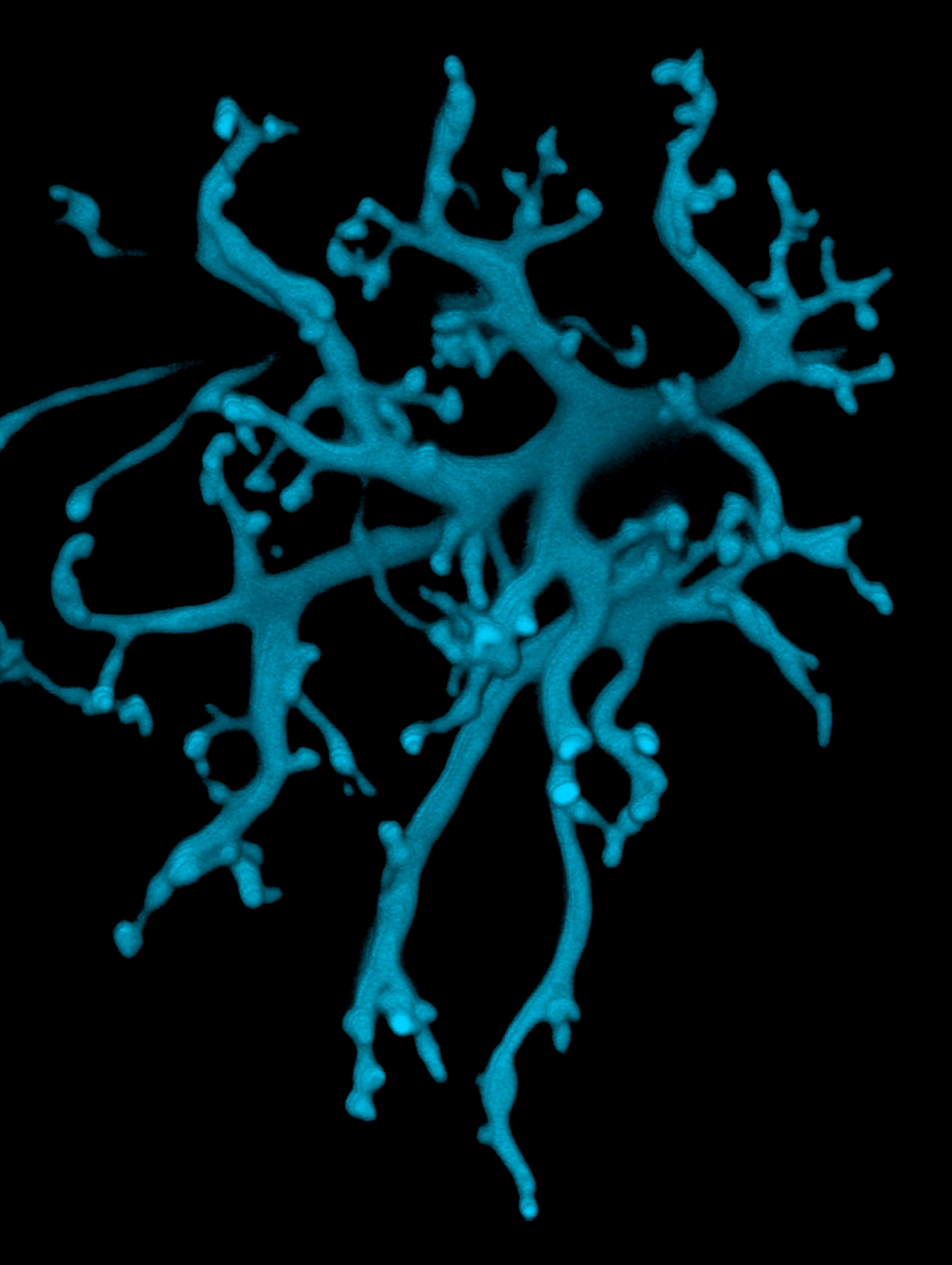
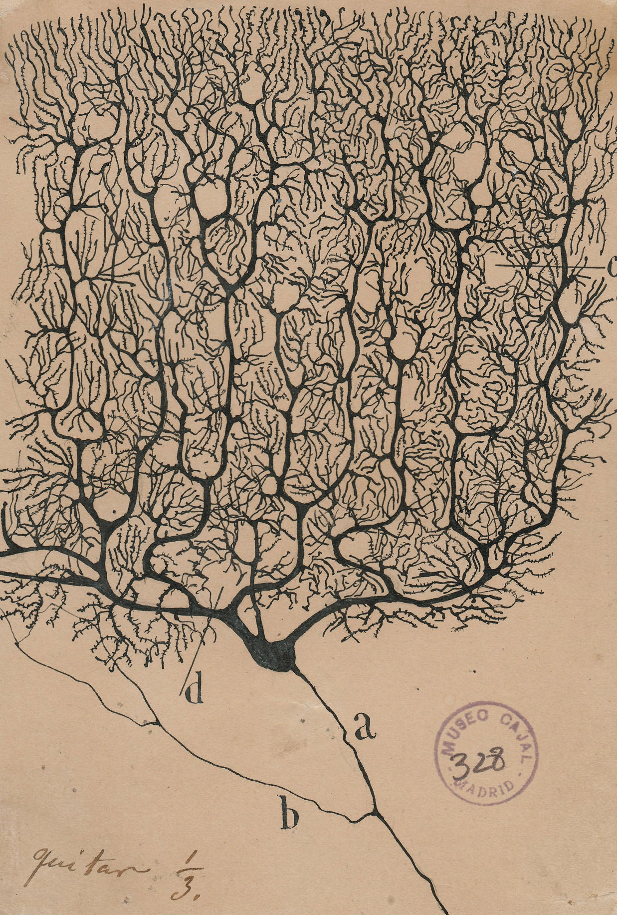
A Purkinje cell dendritic tree (as drawn by Ramón y Cajal) works completely differently than a bipolar cell dendritic tree (as drawn by a computer in blue).
Now we consider spatial summation. Because the small IPSPs and EPSPs decrement over distance (i.e. in space) as they travel from the site where they’re generated (the postsynaptic membrane), they are different sizes by the time they reach their common branch point. The branch point summarizes the “total” of the positive and negative deflections (EPSPs and IPSPs, now smaller than when they began) and reports out the total. That total then joins the totals from other branches, and these meet at a new branch point, and the process continues until we get to the synapse or initial segment.
The decrement in voltage over distance is described by the length constant (λ) which was explained in the blue oval under Objective 6. You still don’t need to know it.
Temporal summation works basically the same way. Synaptic inputs which are closely spaced in time add together: if 5 synapses each see a 3 mV deflection at the exact same time (i.e. within a millisecond), then the total will be close to 15 mV, or above threshold for most neurons.
Each of the incoming EPSPs and IPSPs decrement in time according to the value of the time constant (τ). τ is the time it takes for the voltage to decrement to 1/2.718 of its initial value, as explained for the length constant (λ) in the oval on p. 13-29. You still don’t need to know the numbers, just the idea that graded potentials decrement over distance and decrement over time.
If there is even a slight difference in the arrival of these graded potentials, they won’t sum up perfectly. But they can still act together to trigger an action potential, as shown in this diagram.
The geometry of the neuron determines its function. This is another example of what we’ve been talking about since Unit 1: form and function, anatomy and physiology, are interrelated and interdependent. The shape and arrangement of its dendrites, cell body, and axon, is a reflection of its information processing capabilities, and the information processing capabilities are set by its geometry.
When IPSPs and EPSPs are close to the “decision point” (initial segment or synapse), they have a stronger influence. They can be close in space (spatial summation) or close in time (temporal summation) or both. When threshold is reached, either the threshold for firing an action potential or the threshold for synaptic release, then something happens.
Now imagine 80 billion neurons each of which is hooked up in 10,000 different ways and you begin to appreciate the immense information processing power of the human brain.
Media Attributions
- U11-002 Synapses onto Neuron © NICHD/T. Ahmed, A. Buonanno is licensed under a CC BY-NC-ND (Attribution NonCommercial NoDerivatives) license
- U13-082 Table Action Potentials vs Graded Potentials © Hutchins, Jim and Bizzell, Lizz is licensed under a CC BY-SA (Attribution ShareAlike) license
- U13-083 Postsynaptic Potential Graphs © Wade, Alexia is licensed under a CC BY-SA (Attribution ShareAlike) license
- U13-084 Information Flow in Neurons © Hutchins, Jim is licensed under a CC BY-SA (Attribution ShareAlike) license
- U13-085 Information Flow in Neurons 2 © Hutchins, Jim is licensed under a CC BY-SA (Attribution ShareAlike) license
- U13-086 Bipolar Cell Dendritic Tree © Wei Li, National Eye Institute, Natoinal Institutes of Health is licensed under a CC BY-NC (Attribution NonCommercial) license
- U11-028 Purkinje Cell © Santiago Ramón y Cajal is licensed under a Public Domain license
